Signal detection theory: Yes-no task, normal model unequal variance
Assumed distributions of signal and noise
\(X_n \sim N(0,1) =f_n(x | \theta=0)= \frac{1}{\sqrt{2\pi}}e^{-\frac{x^2}{2}}\)
\(X_s \sim N(d',1) =f_s(x | \theta=d')= \frac{1}{\sqrt{2\pi}\sigma}e^{-\frac{(x-d')^2}{2 \sigma^2}}\)
Example
library(tidyverse)
dprime <- 1
sigma <- 2
x <-  seq(-5, 5, .1)

dist_dat <- tibble(x) %>%
  mutate(f_s = dnorm(x, dprime, sigma),
         f_n = dnorm(x, 0, 1))

p <- dist_dat %>%
  ggplot() +
  geom_line(aes(x = x, y = f_s, lty = "signal")) +
  geom_line(aes(x = x, y = f_n, lty = "noise")) +
  labs(y = "f")
p
Likelihood
\[\log{\Lambda}(x) = -\frac{1}{2\sigma^2} \left( (1-\sigma^2) x^2 - 2d'x+d'^2+2\sigma^2\log(\sigma) \right) \]
Example
ll_fun <- function(x, p) - 1 / (2 * p[2]^2) * ( (1 - p[2]^2) * x^2 - 2 * p[1] * x + p[1]^2 +2*p[2]^2*log(p[2]) )

ll <- tibble(x) %>%
  mutate(ll = ll_fun(x, c(dprime, sigma)))

ll %>%
  ggplot() +
geom_line(aes(x = x, y = ll)) 
It can be seen that the log likelihood is non-monotonic on x. For large positive and negative values of x, it is more likely that the state of the world was signal, rather than noise.
Decision rule
For \(\log{\Lambda}(x) > \lambda\) choose \(a_S\)
results in
\[-\frac{1}{2\sigma^2} \left( (1-\sigma^2) x^2 - 2d'x+d'^2+2\sigma^2\log(\sigma) + 2\sigma^2 \lambda \right) > 0\] \[ (1-\sigma^2) x^2 - 2d'x+d'^2+2\sigma^2 (\log(\sigma) + \lambda) < 0\] When \(\sigma > 1\), the decision rule is
\[\text{If } x < c_1 \, \text{ or } \, x > c_2 \text{ then }a=a_S\] \[\text{If } c_1 < x < c_2 \text{ then }a=a_N\]
When \(\sigma < 1\), the decision rule is
\[\text{If } x < c_1 \, \text{ or } \, x > c_2 \text{ then }a=a_N\]
\[\text{If } c_1 < x < c_2 \text{ then }a=a_S\]
where \(c_1\) and \(c_2\) are given by
\[c_1 = \frac{d'+\sqrt{d'^2-(1-\sigma^2)(d'^2+2\sigma^2(log(\sigma) + \lambda))}}{1-\sigma^2}\] \[c_2 = \frac{d'-\sqrt{d'^2-(1-\sigma^2)(d'^2+2\sigma^2(log(\sigma) + \lambda))}}{1-\sigma^2}\] We can use the sensory space to decide, but there are 2 relevant criteria. The observer model is completely specified by \(d'\), \(\sigma\) and \(\lambda\). For the model to be identifiable, we need that the observer performs the task using at least two criteria.
Notice that for having real solutions \(\lambda\) should be larger that the minimun of the log likelihood.
Example
For the proposed example, let’s calculate \(c_1\) and \(c_2\) in the sensory space for different likelihood criteria including the ideal observer (\(\lambda=0\))
calculate_c1_c2 <- function(.dprime, .sigma, .lambda) {
  sqr_root <- sqrt(.dprime^2 - (1-.sigma^2)*(.dprime^2 + 2*.sigma^2*(log(.sigma) + .lambda)))

  c1 <- (.dprime + sqr_root) / (1 - .sigma^2)
  c2 <- (.dprime - sqr_root) / (1 - .sigma^2)

  tibble(c1, c2)
}

c1_c2 <- tibble(lambda = c(-0.8595, -0.8, -0.5 , 0, 1, 3)) %>%
  group_by(lambda) %>%
  summarise(calculate_c1_c2(dprime, sigma, lambda))
## `summarise()` ungrouping output (override with `.groups` argument)p +
geom_vline(data = c1_c2, aes(xintercept = c1, color = factor(lambda))) +
geom_vline(data = c1_c2, aes(xintercept = c2, color = factor(lambda)))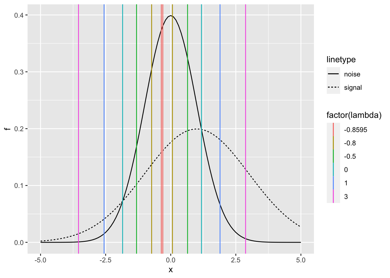
For the ideal obsercer, \(c_1\) and \(c_2\) corresponds to the intersections of the two distributions.
You can compute \(c_1\) and \(c_2\) also using the function UVGSDTcrit from the book Modelling Psychophysical data in R
UVGSDTcrit <- function(dp, sig, logbeta){
  TwoSigSq <- 2 * sig^2
  minLam <- optimize(function(X, dp, sig)
  -((1 - sig^2) * X^2 - 2 * dp * X +
      dp^2 + TwoSigSq * log(sig))/TwoSigSq, c(-10, 10),
      dp = dp, sig = sig)$objective
  if (logbeta < minLam) warning("complex roots")
  cf <- -c(dp^2 + TwoSigSq * log(sig) + logbeta *
             TwoSigSq,
           -2 * dp, 1 - sig^2)/TwoSigSq
  proot <- polyroot(cf)
  sort(Re(proot))
}
For example, for the optimal criterion
UVGSDTcrit(dprime, sigma, 0)## [1] -1.847545 1.180878Probabilities
Under the 0-1 loss model, the observer model can be reparametrized in terms of the probabilities. Let’s consider the situation \(\sigma >1\)
\(p_{FA}=P(a_S|H_N)=\int_{x \in R} f_n(x) \,dx = 1 - \left(\Phi(c_2)- \Phi(c_1)\right)\)
\(p_{H}=P(a_S|H_N)=\int_{x \in R} f_s(x) \,dx = 1 - \left( \Phi\left(\frac{c_2-d'}{\sigma}\right) - \Phi \left(\frac{c_1-d'}{\sigma}\right) \right)\)
ROC
Let’s plot the ROC curve for the previous example
c1_c2_roc <- c1_c2 %>%
  mutate(p_fa = 1 - (pnorm(c2) - pnorm(c1)),
         p_h = 1 - (pnorm(c2, dprime, sigma) - pnorm(c1, dprime, sigma)))

p_c1_c2_roc <- c1_c2_roc %>%
  ggplot() +
  geom_line(aes(x = p_fa, y = p_h)) +
  geom_point(aes(x = p_fa, y = p_h, color = factor(lambda))) +
  geom_segment(color = "grey", aes(x = 0, y = 0, xend = 1, yend = 1)) +
  xlim(0, 1) +
  ylim(0, 1)

p_c1_c2_roc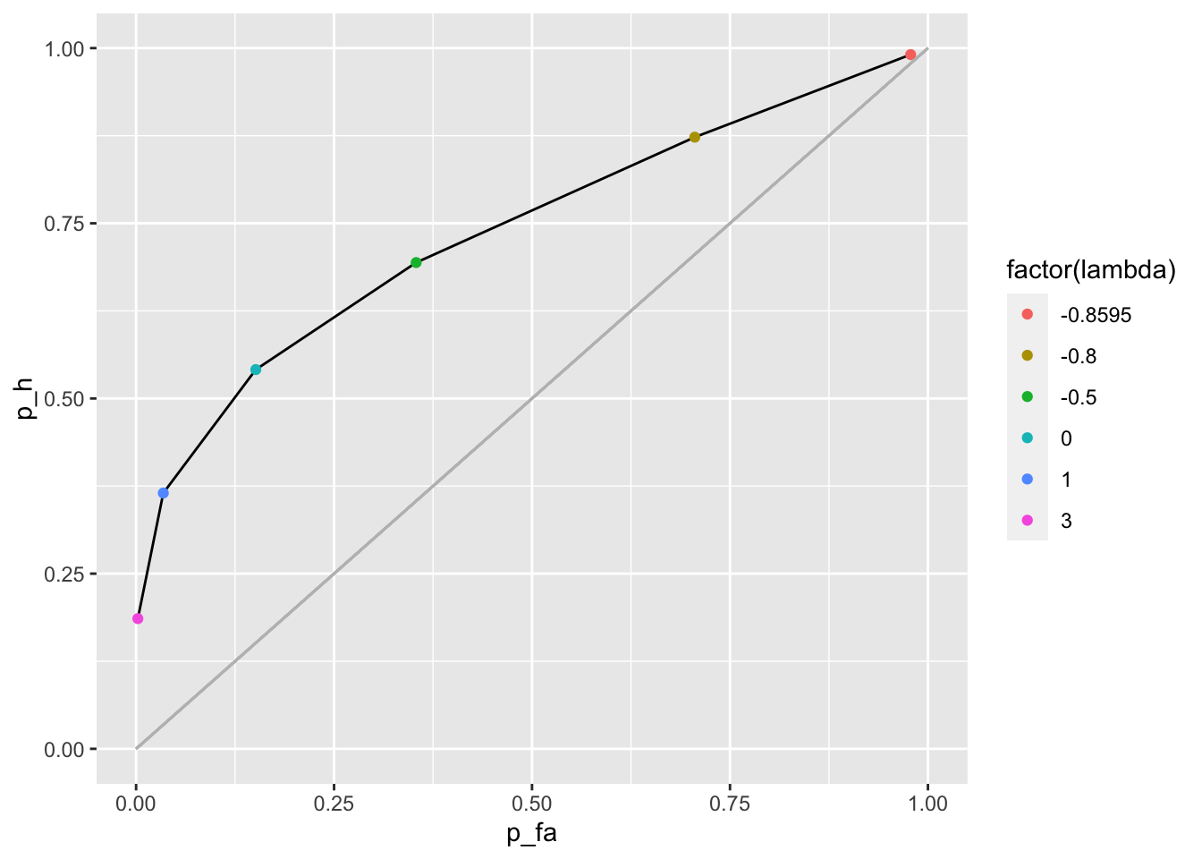
As expected the criterion \(\lambda = 0\) maximizes correct responses
c1_c2_roc %>%
    mutate(p_m = 1 - p_h,
           p_cr = 1 - p_fa,
           p_correct = .5 *(p_h + p_cr))
## # A tibble: 6 x 8
## lambda c1 c2 p_fa p_h p_m p_cr p_correct
## * <dbl> <dbl> <dbl> <dbl> <dbl> <dbl> <dbl> <dbl>
## 1 -0.860 -0.362 -0.304 0.978 0.991 0.00924 0.0218 0.506
## 2 -0.8 -0.733 0.0660 0.706 0.873 0.127 0.294 0.584
## 3 -0.5 -1.31 0.646 0.354 0.694 0.306 0.646 0.670
## 4 0 -1.85 1.18 0.151 0.541 0.459 0.849 0.695
## 5 1 -2.56 1.89 0.0344 0.365 0.635 0.966 0.665
## 6 3 -3.54 2.87 0.00222 0.186 0.814 0.998 0.592ROC using a sensory criterion
Let’s suppose that the observer, instead of using a likelihood criterion uses a criterion in the sensory evidence
\(p_{FA} = 1 - \Phi(c)\)
\(p_{H} = 1 - \Phi\left(\frac{c-d'}{\sigma}\right)\)
c1_c2_roc_sensory_crit <- tibble(crit = seq(-10, 10, .1)) %>%
  mutate(p_fa = 1 - pnorm(crit),
         p_h = 1 - pnorm(crit, dprime, sigma))

p_c1_c2_roc  +
  geom_line(data = c1_c2_roc_sensory_crit, aes(x = p_fa, y = p_h, lty = "sensory criterion")) +
  scale_linetype_manual(values = 2)
The model predicts that for large proportion of false alarms, this prorportion is larger than proportion of hits.
Notice that if we use a more moderate value for \(\sigma\) the ROC curves for the likelihood and sensory criterion are very similar
c1_c2_roc_smaller_sigma <- tibble(lambda = c(-0.8, -0.8, -0.5 , 0, 1, 3)) %>%
  group_by(lambda) %>%
  summarise(calculate_c1_c2(dprime, 1.5, lambda)) %>% # sigma = 1.5
  mutate(p_fa = 1 - (pnorm(c2) - pnorm(c1)),
         p_h = 1 - (pnorm(c2, dprime, sigma) - pnorm(c1, dprime, sigma)))
## `summarise()` regrouping output by 'lambda' (override with `.groups` argument)c1_c2_roc_sensory_crit_smaller_sigma <- tibble(crit = seq(-10, 10, .1)) %>%
mutate(p_fa = 1 - pnorm(crit),
p_h = 1 - pnorm(crit, dprime, 1.5)) # sigma = 1.5
c1_c2_roc_smaller_sigma %>%
ggplot() +
geom_line(aes(x = p_fa, y = p_h)) +
geom_point(aes(x = p_fa, y = p_h, color = factor(lambda))) +
geom_segment(color = "grey", aes(x = 0, y = 0, xend = 1, yend = 1)) +
geom_line(data = c1_c2_roc_sensory_crit_smaller_sigma, aes(x = p_fa, y = p_h, lty = "sensory criterion")) +
scale_linetype_manual(values = 2) +
xlim(0, 1) +
ylim(0, 1) 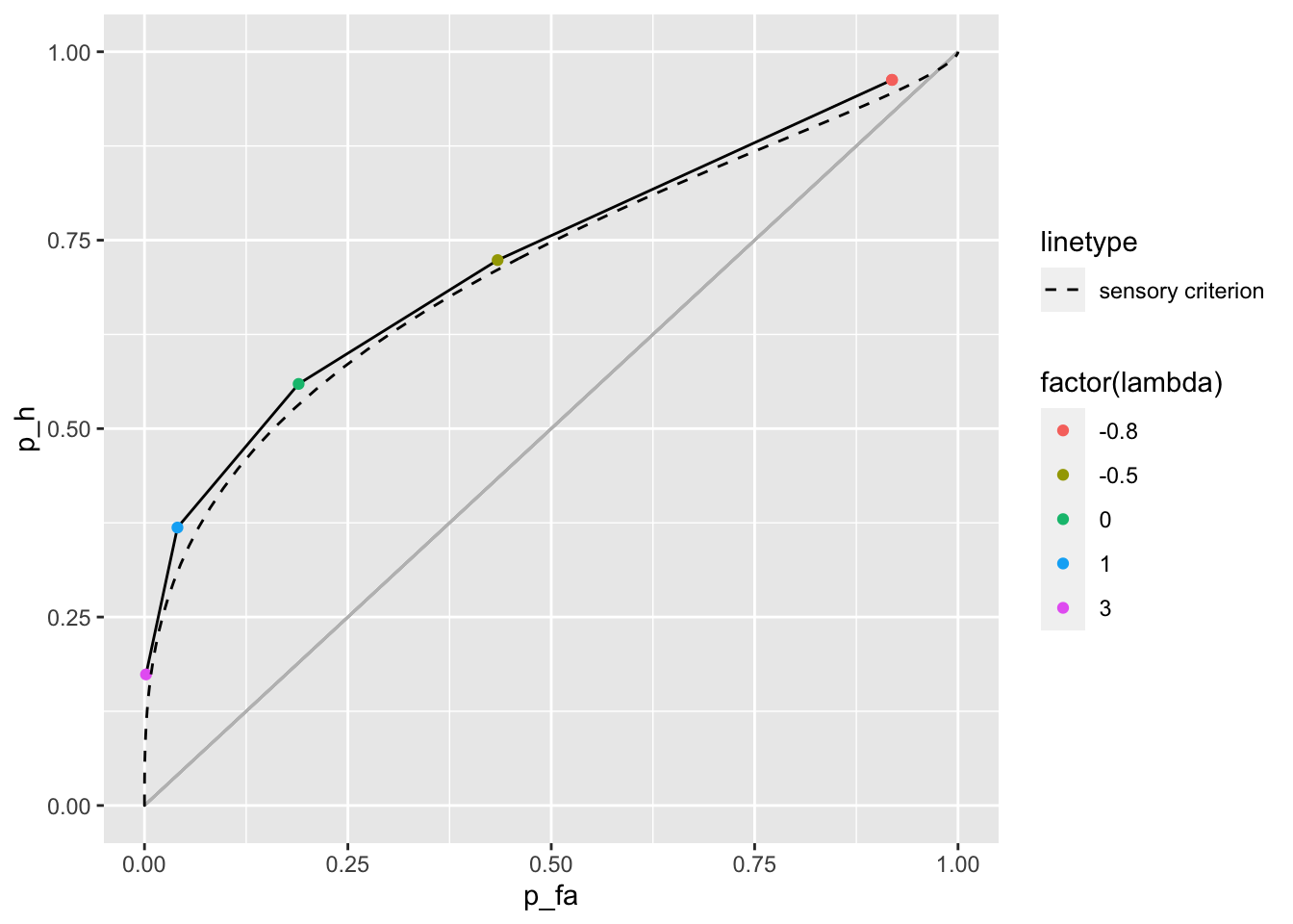
Slope in ROC and likelihood at criterion
The slope in ROC is the likelihood at criterion independently of the decision rule used
slope_loglik_crit <- tibble(lambda = seq(-0.8595, 3, 0.005)) %>%
  group_by(lambda) %>%
  summarise(calculate_c1_c2(dprime, sigma, lambda)) %>%
  mutate(p_fa = 1 - (pnorm(c2) - pnorm(c1)),
         p_h = 1 - (pnorm(c2, dprime, sigma) - pnorm(c1, dprime, sigma)),
         lik = exp(ll_fun(c1, c(dprime, sigma))),
         slope = ( lag(p_h) - p_h) / (lag(p_fa) - p_fa)) %>%
  select(p_fa, p_h, lik, slope) %>%
  mutate(cond = "loglik crit")
## `summarise()` ungrouping output (override with `.groups` argument)slope_sensory_crit <- tibble(crit = seq(-3, 3, .05)) %>%
mutate(p_fa = 1 - pnorm(crit),
p_h = 1 - pnorm(crit, dprime, sigma),
lik = exp(ll_fun(crit, c(dprime, sigma))),
slope = ( lag(p_h) - p_h) / (lag(p_fa) - p_fa)) %>%
select(p_fa, p_h, lik, slope) %>%
mutate(cond = "sensory crit")
slope_loglik_crit %>%
bind_rows(slope_sensory_crit) %>%
ggplot()+
geom_segment(color = "grey", aes(x = 0, y = 0, xend = 1, yend = 1)) +
geom_line(aes(x = p_fa, y =p_h, color = cond, size = "ROC")) +
geom_line(aes(x = p_fa, y = lik, color = cond, lty = "likelihood at criterion", size = "SLOPES")) +
geom_line(aes(x = p_fa, y = slope, color = cond, lty = "slope", size = "SLOPES")) +
scale_size_manual(values = c(2, .5)) +
coord_cartesian(xlim = c(0, 1), y = c(0, 1))## Warning: Removed 2 row(s) containing missing values (geom_path).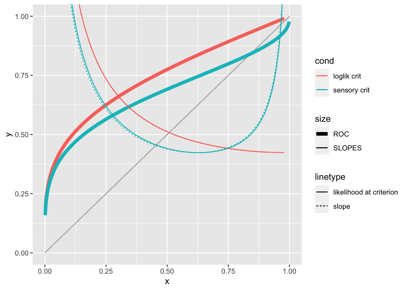
zROC
The zROC curve is a straight line only for the decision rule using the sensory criterion.
\(p_{FA} = 1 - \Phi(c) = \Phi(-c)\)
\(p_{H} = 1 - \Phi(\frac{c-d'}{\sigma}) = \Phi(\frac{d'-c}{\sigma})\)
then
\(\Phi^{-1}(p_{FA}) = -c\)
\(\Phi^{-1}(p_{H}) = \frac{d'-c}{\sigma}\)
That is
\(\Phi^{-1}(p_{H}) = \frac{1}{\sigma}d' + \frac{1}{\sigma}\Phi^{-1}(p_{FA})\)
The slope is \(1 / \sigma\) and the intercept is \(d' / \sigma\).
library(cowplot)

plot_grid(
  slope_loglik_crit %>%
  bind_rows(slope_sensory_crit) %>%
  ggplot()+
  geom_segment(color = "grey", aes(x = 0, y = 0, xend = 1, yend = 1)) +
  geom_line(aes(x = p_fa, y =p_h, color = cond)) +
  coord_equal() +
  theme(legend.position = "top")
  ,
  slope_loglik_crit %>%
  bind_rows(slope_sensory_crit) %>%
  mutate(z_fa = qnorm(p_fa),
         z_h = qnorm(p_h)) %>%
  ggplot()+
  geom_line(aes(x = z_fa, y =z_h, color = cond)) +
  coord_equal() +
  theme(legend.position = "top")
)