model_selection
To perform model selection, the dev version of quickspy is necessary.
Model selection is quite flexible in quickpsy as in the fun argument you can introduce any arbitrary set of functions with all possible combinations of shared parameters (see the last subsection of the functions section)
To perform model selection, quickpsy uses likelihood ratio tests and the Akaike Information Criterion (see References).
Model 1
Let’s fit a model for each participant in which the slope does not change across conditions
library(quickpsy)
library(dplyr)

# the shared parameter is p[2]
fun_1_df <- tibble(cond = c("cond1", "cond2"),
                   fun = c(function(x, p) pnorm(x, p[1], p[2]),
                           function(x, p) pnorm(x, p[3], p[2])))

fit_1 <- quickpsy(qpdat, phase, resp,
                  grouping = c("participant", "cond"),
                  fun = fun_1_df,
                  parini = c(-100, 50, -100),
                  bootstrap = "none")

plot(fit_1, color = cond)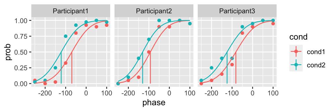
We can look at the likelihoods of the models
fit_1$logliks
#> # A tibble: 3 x 3
#> # Groups:   participant [3]
#>   participant  loglik n_par
#>   <chr>         <dbl> <int>
#> 1 Participant1  -44.8     3
#> 2 Participant2  -26.5     3
#> 3 Participant3  -23.0     3
or the AICs
fit_1$aic
#> # A tibble: 3 x 3
#> # Groups:   participant [3]
#>   participant    aic n_par
#>   <chr>        <dbl> <int>
#> 1 Participant1  95.6     3
#> 2 Participant2  59.0     3
#> 3 Participant3  52.0     3
Model 2
Now let’s fit a model in which for each participant the slope can change across conditions
fun_2_df <- tibble(cond = c("cond1", "cond2"),
                   fun = c(function(x, p) pnorm(x, p[1], p[2]),
                           function(x, p) pnorm(x, p[3], p[4])))

fit_2 <- quickpsy(qpdat, phase, resp,
                  grouping = c("participant", "cond"),
                  fun = fun_2_df,
                  parini = c(-100, 50, -100, 50),
                  bootstrap = "none")

plot(fit_2, color = cond)
Model selection: likelihood ratio test
The quickpsy function model_selection_lrt performs the likelihood ratio tests using the chi square distribution. The inputs are the likelihoods of each model.
model_selection_lrt(fit_1$logliks, fit_2$logliks)
#> # A tibble: 3 x 8
#> # Groups:   participant [3]
#>   participant  loglik1 n_par1 loglik2 n_par2 deviance p.value best
#>   <chr>          <dbl>  <int>   <dbl>  <int>    <dbl>   <dbl> <chr>
#> 1 Participant1   -44.8      3   -43.1      4  3.44     0.0637 first
#> 2 Participant2   -26.5      3   -26.5      4  0.00720  0.932  first
#> 3 Participant3   -23.0      3   -22.7      4  0.487    0.485  first
Using the default 5% criterion of significance, the Model 2 (allowing a different slope for each condition) does not improve the fit for any participant. There is some evidence, however, that for Participant 1 the Model 2 might be better.
Model selection: Akaike Information Criterion
To perform the model selection using quickpsy, you need to introduce in the model_selection_aic function the AICs of each model.
model_selection_aic(fit_1$aic, fit_2$aic)
#> # A tibble: 3 x 7
#> # Groups:   participant [3]
#>   participant   aic1 n_par1  aic2 n_par2     p best
#>   <chr>        <dbl>  <int> <dbl>  <int> <dbl> <chr>
#> 1 Participant1  95.6      3  94.2      4 0.237 second
#> 2 Participant2  59.0      3  61.0      4 7.34  first
#> 3 Participant3  52.0      3  53.5      4 4.54  first
Using Akaike Information Criterion the Model 1 is preferred for Participant 2 and 3 and the Model 2 is preferred for Participant 1. The p indicates the relative probability of each model.
References
Kingdom FAA, Prins N. 2016. Psychophysics: A Practical Introduction. Elsevier Science.
Knoblauch, K., & Maloney, L. T. (2012). Modeling psychophysical data in R (Vol. 32). Springer Science & Business Media.
Prins, N. (2018). Applying the model-comparison approach to test specific research hypotheses in psychophysical research using the Palamedes toolbox. Frontiers in psychology, 9, 1250.