Hypothesis testing
Definition of hypotheses
A hypothesis is a statement about a population parameter.
\[H_0: \theta \in \Theta_0 \text{ and } H_1: \theta \in \Theta_1\]
Often \(\Theta_1 = \Theta_0^C\).
Types of hypotheses
Simple hypothesis
\[H_0: \theta = \theta_0\]
Composite hypothesis
When the hypothesis is not simple.
Types of hypothesis test
Simple
\[H_0: \theta = \theta_0 \text{ and } H_1: \theta = \theta_1\]
Composite
One-side
\[H_0: \theta \leq \theta_0 \text{ and } H_1: \theta > \theta_0\]
or
\[H_0: \theta \geq \theta_0 \text{ and } H_1: \theta > \theta_0\]
Two-sides
\[H_0: \theta = \theta_0 \text{ and } H_1: \theta \neq \theta_0\]
That is, under \(H_1\), \(\theta = (\theta_1,\dotsc,\theta_m,\theta_{m+1},\dotsc,\theta_{m+p})\) and under \(H_0\), \(\theta = (\theta_1,\dotsc,\theta_m,\theta_{m+1}=\theta_{0,1},\dotsc,\theta_{m+p}=\theta_{0,p})\).
Action space
\(\mathcal{A} = \{ a_0, a_1\}\) where \(a_0\) represents choosing \(H_0\) and \(a_1\) represents choosing \(H_1\)
Decision rule
In the context of hypothesis testing, a decision rule is called hypothesis test and it is defined by the sample values \(x\) for which we accept or reject \(H_0\). The sample values for which we reject \(H_0\) is called the rejection region \(R\).
\(d(x) = \left\{ \begin{array}{ll} a_0 \ if \ x \not\in R \\ a_1 \ if \ x \in R \\ \end{array} \right.\)
The rejection region is often specified by establishing a criterium on a test statistic \(W(x)\) (function of the sample):
\[R=\{x: W(x)<c\}\]
A common method to find a test statistic is the likelihood ratio. To completely specify \(R\), we need \(c\) which can be obtained by setting the probabilities of making mistakes.
Example
\(d(x) = \left\{ \begin{array}{ll} a_0 \ if \ \overline{x} \leq 4.3 \\ a_1 \ if \ \overline{x} > 4.3 \\ \end{array} \right.\)
Evaluating tests (probabilities of making mistakes)
Type I error: \(H_0\) is true \((\theta \in \Theta_0)\) and \(a=a_1\).
Type II error: \(H_1\) is true \((\theta \in \Theta_1)\) and \(a=a_0\).
There are 4 interesting probabilities:
\(P(a_1 | H_0) = P (Type \,I\, error)\)
\(P(a_1 | H_1)\)
\(P(a_0 | H_0)\)
\(P(a_0 | H_1) = P (Type \, II \, error)\)
Power function of a test (power function of a rejection region)
\[\beta(\theta) = P_\theta (X \in R)\]
A good test should have \(\beta(\theta)\) near 0 when \(\theta \in \Theta_0\) and near 1 when \(\theta \in \Theta_1\).
Example 1
\(X \sim B(5,p)\)
\(H_0: p \leq 1/2\)
\(H_1: p > 1/2\)
\(R=\{k = 5 \}\)
\(\beta(p) = P_p(k \in R) = P_p(k = 5) = \binom{5}{5} p^5 (1-p)^0 = p^5\)
library(ggplot2)## Warning in file(con, "r"): cannot open file '/var/db/timezone/zoneinfo/
## +VERSION': No such file or directoryp <- seq(0,1,.01)
beta <- p^5
dat <- data.frame(p,beta)
ggplot(dat,aes(x=p,y=beta))+geom_line()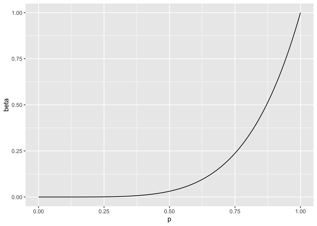
The probability of Type II error is quite large.
\(R=\{k \geq 3 \}\)
\(\beta(p) = P_p(k \in R) = P_p(k = 3 \ or \ k = 4 \ or \ k =5 ) = \binom{5}{3} p^3 (1-p)^2 + \binom{5}{4} p^4 (1-p)^1 + \binom{5}{5} p^5(1-p)^0\)
p <- seq(0,1,.01)
beta <- 10*p^3*(1-p)^2 + 5*p^4*(1-p)+p^5
dat <- data.frame(p,beta)
ggplot(dat,aes(x=p,y=beta))+geom_line()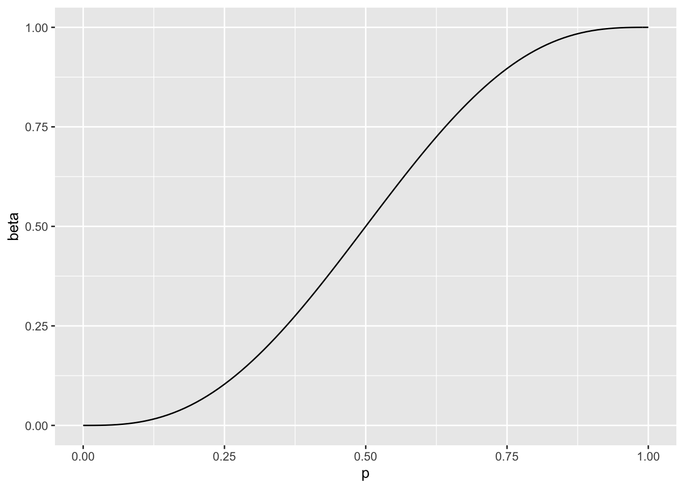
The Type II error decreases, but Type I increases.
Size \(\alpha\) of a test
\[sup_{\theta \in \Theta_0} \beta(\theta) = \alpha\]
In example 1, \(\alpha\)s are respectively
p <- .5
p^5
## [1] 0.0312510*p^3*(1-p)^2 + 5*p^4*(1-p)+p^5## [1] 0.5Level \(\alpha\) of a test
\[sup_{\theta \in \Theta_0} \beta(\theta) \leq \alpha\]
Null hypothesis testing
\(H_0\) and \(H_1\) are treated asymmetrically as \(\alpha\) is fixed (often to .01 or .05) so that the Type I error is less than \(\alpha\).
UMP
A test in class \(\mathcal{C}\) with a power function \(\beta(\theta)\) is the uniformly most powerful (UMP) test of class \(\mathcal{C}\) if \(\beta(\theta) \geq \beta'(\theta)\) for all \(\theta \in \Theta_1\).
UMP level \(\alpha\)
\(\mathcal{C} = \text{ all level } \alpha \text{ tests}\).
p-value
A p-value \(p(X)\) is a test statistics that satisfies \[0 \leq p(X) \leq 1\]
It is valid if \[P_{\theta} \left( p \left( X \right) \leq \alpha\right) \leq \alpha\]
Loss and risk functions
0-1
\(L(\theta,a) = \left\{ \begin{array}{ll} 1 & \mbox{if } \theta \in \Theta_0 \text{ and } a=a_1\\ 1 & \mbox{if } \theta \in \Theta_1 \text{ and } a=a_0 \\ 0 & \text{otherwise} \\ \end{array} \right.\)
\(R(\theta,d) = \left\{ \begin{array}{ll} P_{\theta\ \in \Theta_0}\left(d(X)=a_1\right) =\beta(\theta) & \mbox{if } \theta \in \Theta_0 \\ P_{\theta\ \in \Theta_1}\left(d(X)=a_0\right) =1 -\beta(\theta) & \mbox{if } \theta \in \Theta_1 \\ \end{array} \right.\)
Demonstration
If \(\theta \in \Theta_0\)
\(R(\theta,d(X)) = \int_R L(\theta,d(X)) f(x; \theta) \, dx + \int_{R^C} L(\theta,d(X)) f(x; \theta) \, dx = \int_R L(\theta,a_1) f(x; \theta) \, dx + \int_{R^C} L(\theta,a_0) f(x; \theta) \, dx= \\ = \int_R 1 \, f(x; \theta) \, dx + \int_{R^C} 0 \, f(x; \theta) \, dx = \int_R f(x; \theta) \, dx = P_{\theta\ \in \Theta_0}(d(X)=a_1)\)
If \(\theta \in \Theta_1\)
\(R(\theta,d(X)) = \int_R L(\theta,d(X)) f(x; \theta) \, dx + \int_{R^C} L(\theta,d(X)) f(x; \theta) \, dx = \int_R L(\theta,a_1) f(x; \theta) \, dx + \int_{R^C} L(\theta,a_0) f(x; \theta) \, dx= \\ = \int_R 0 \, f(x; \theta) \, dx + \int_{R^C} 1 \, f(x; \theta) \, dx = \int_{R^C} f(x; \theta) \, dx = P_{\theta\ \in \Theta_1}(d(X)=a_0)\)
Example
p <- seq(0,1,.01)
risk <- ifelse(p<.5, p^5, 1 - p^5)
dat <- data.frame(p,risk)
ggplot(dat,aes(x=p,y=risk))+geom_line()
Generalised 0-1
\(L(\theta,a) = \left\{ \begin{array}{ll} c_I & \mbox{if } \theta \in \Theta_0 \text{ and } a=a_1\\ c_{II} & \mbox{if } \theta \in \Theta_1 \text{ and } a=a_0 \\ 0 & \text{otherwise} \\ \end{array} \right.\)
\(R(\theta,d) = \left\{ \begin{array}{ll} P_{\theta\ \in \Theta_0}\left(d(X)=a_1\right) =c_I \beta(\theta) & \mbox{if } \theta \in \Theta_0 \\ P_{\theta\ \in \Theta_1}\left(d(X)=a_0\right) =c_{II} \left( 1 -\beta(\theta) \right) & \mbox{if } \theta \in \Theta_1 \\ \end{array} \right.\)
More general
\(L(\theta,a) = \left\{ \begin{array}{ll} -V_{00} & \mbox{if } \theta \in \Theta_0 \text{ and } a=a_0\\ V_{01} & \mbox{if } \theta \in \Theta_0 \text{ and } a=a_1\\ -V_{11} & \mbox{if } \theta \in \Theta_1 \text{ and } a=a_1\\ V_{10} & \mbox{if } \theta \in \Theta_1 \text{ and } a=a_0\\ \end{array} \right.\)
\(R(\theta,a) = \left\{ \begin{array}{ll} V_{10} P_{\theta\ \in \Theta_0}\left(d(X)=a_1\right) - V_{00} P_{\theta\ \in \Theta_0}\left(d(X)=a_0\right)& \mbox{if } \theta \in \Theta_0 \\ V_{01} P_{\theta\ \in \Theta_1}\left(d(X)=a_0\right) - V_{11} P_{\theta\ \in \Theta_1}\left(d(X)=a_1\right) & \mbox{if } \theta \in \Theta_1 \\ \end{array} \right.\)
References
Casella, G., & Berger, R. L. (2002). Statistical inference (Vol. 2). Duxbury Pacific Grove, CA.
Wasserman, L. (2013). All of statistics: A concise course in statistical inference. Springer Science & Business Media.
Young, G. A., & Smith, R. L. (2005). Essentials of statistical inference (Vol. 16). Cambridge University Press.