functions
Predefined functions
quickpsy incorporates 3 predefined functions to characterize the shape of the psychometric function: cum_normal_fun, logistic_fun and weibull_fun.
Let’s see, for example, the definition of the logistic_fun
library(quickpsy)
logistic_fun
#> function(x, p) (1 + exp(-p[2] * (x - p[1])))^(-1)
#> <bytecode: 0x7fbef2353a90>
#> <environment: namespace:quickpsy>
By default, quickspy fits cum_normal_fun, but you can change the function using the fun argument
fit <- quickpsy(qpdat, phase, resp, grouping = c("participant", "cond"),
                fun = logistic_fun, bootstrap = "none")

plot(fit, color = cond)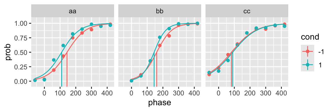
You can see that it is not necessary to include initial parameters to fit a predefined function.
Functions defined by the user
In the fun argument you can incorporate any function. For non-predefined functions you need to include initial parameters.
gompertz_fun <- function(x, p) exp(-p[1] * exp(-p[2] * x))

fit <- quickpsy(qpdat, phase, resp, grouping = c("participant", "cond"),
                fun = gompertz_fun, parini = c(0.1, 0.02), bootstrap = "none")

plot(fit)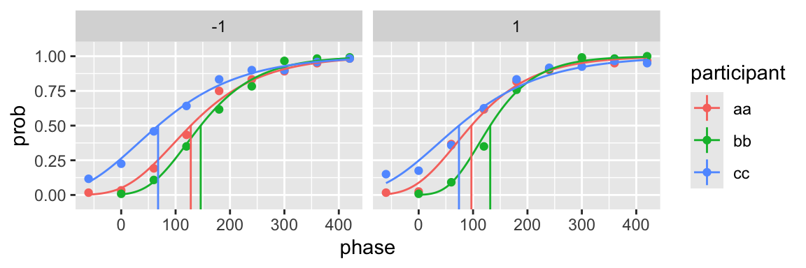
The function does not need to be monotonic
n <- 100
x <- seq(-.3, .3, .1)
k <- c(10, 45, 90, 100, 60, 10, 5)
dat <- data.frame(x, k, n)

gaussian <- function(x, p) exp(-0.5*((x - p[2]) / p[3])^2) / (1 + exp(-p[1]))

fit <- quickpsy(dat, x, k, n, fun = gaussian, parini = c(0, 0, 0),
                thresholds = FALSE, # because the threshold is not well defined
                bootstrap = "none")
plot(fit)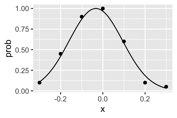
Data frame of functions (dev version of quickpsy)
In the fun argument you can also incorporate a data frame of functions specifying with function you want to fit to every condition (the data frame should be a tibble to support lists of functions).
One advantage of this approach is that you can easily specify shared parameters across conditions, such as the slope parameter in the following example using the logistic function
library(dplyr)

fun_df <- tibble(cond = c("cond1", "cond2"),
                 fun = c(function(x, p) (1 + exp(-p[2] * (x - p[1])))^(-1),
                         function(x, p) (1 + exp(-p[2] * (x - p[3])))^(-1)))

fit <- quickpsy(qpdat, phase, resp, grouping = c("participant", "cond"),
                fun = fun_df,
                parini = c(-100, 0.02, -100),
                bootstrap = "none")

plot(fit, color = cond)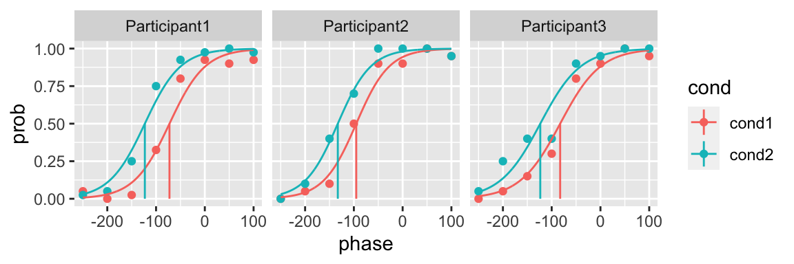
This is another example using a shared leftward and rightward asymptote across conditions using the cumulative normal function
fun_df <- tibble(cond = c("cond1", "cond2"),
                 fun = c(function(x, p) p[5] + (1 - p[5] - p[6]) * pnorm(x, p[1], p[2]),
                         function(x, p) p[5] + (1 - p[5] - p[6]) * pnorm(x, p[3], p[4])))

fit <- quickpsy(qpdat, phase, resp, grouping = c("participant", "cond"),
                fun = fun_df,
                parini = c(-100, 50, -100, 50, 0.01, 0.01),
                bootstrap = "none")

plot(fit, color = cond)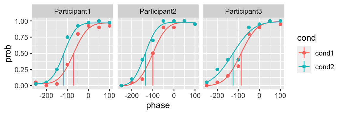
For a given data set you can try different models and then compare them using likelihood ratio tests or the Akaike information criterion (see model_selection section).