Simple linear regression
Definition
Given
\[(Y_1, X_1), (Y_2, X_2),\dots,(Y_n, X_n) \sim F_{Y, X}\]
Our goal is to estimate the regression function defined as
\[r(x) = E[Y|X=x] = \beta_0 + \beta_1x\]
So, the model is completely specified given:
- The probability distribution of \(Y\).
- The relation between the expected values of \(Y\) and a linear combination of the explanatory variables.
Alternative definition
We have \(n\) pairs of random variables in which each pair is
\[Y_i = \beta_0 + \beta_1X_i + \epsilon_i\] with \[E[\epsilon_i|X_i] = 0\]
and
variance that does not depend on \(X_i\)
\[V[\epsilon_i|X_i]=\sigma^2\]
Normal case
Sometimes, it is assumed that the variability is normal
\[\epsilon_i|X_i \sim N(0,\sigma^2)\]
that is,
\[Y_i|X_i \sim N(\mu_i, \sigma^2)\] where \(\mu_i = \beta_0 + \beta_1X_i\).
Explicit form of the statistical model
\[f_{model}(y_1, \cdots, y_n, x_1, \cdots, x_n) = \prod_{i=1}^{n} f(y_i, x_i; \beta_0, \beta_1, \sigma) \]
where
\[f(y, x; \beta_0, \beta_1, \sigma) = \frac{1}{\sqrt{2 \pi} \sigma} \exp{- \frac{(y- \beta_0 -\beta_1x)^2 }{2 \sigma^2}}\]
It is clear from the marginal distribution that the regression function is linear
\[r(x) = E[Y|X=x] = \int_{-\infty}^{\infty} f(y|x) \, dy = \int_{-\infty}^{\infty} y \frac{1}{\sqrt{2 \pi} \sigma} \exp{- \frac{(y- \beta_0 -\beta_1x)^2 }{2 \sigma^2}} \, dy = \beta_0 + \beta_1 x\]
Fitted line
\[\hat{r}(x) = E[Y|X]= \hat{\beta}_0+\hat{\beta}_1x\]
Predicted values
\[\hat{Y}_i = \hat{r}(X_i)\]
Residuals
\[\hat{\epsilon}_i = Y_i -\hat{Y}_i= Y_i - \left( \hat{\beta}_0+\hat{\beta}_1x \right)\]
Residuals sums of squares
\[SS_{res} = \sum_{i=1}^n \hat{\epsilon}_i^2\]
Least squares estimation
The least squares estimates \(\hat{\beta_0}\) and \(\hat{\beta_1}\) are the ones that minimize RSS.
Theorem
\[\hat{\beta_1} = \frac{cov(X, Y)}{V(X)}\] \[\hat{\beta_0} = \overline{Y}_n - \hat{\beta_1}\overline{X}_n \] Unbiased estimat of \(\sigma\)
\[\hat{\sigma} = \frac{SS_{res}}{n-2}\]
Example
library(tidyverse)

x<- c(.2, .4, .6, .8, 1)
y <- c(1, 2.3, 3, 3.5, 4.9)
dat <- data.frame(x, y)

p <- ggplot()+
  geom_point(data = dat,aes(x = x, y = y))
p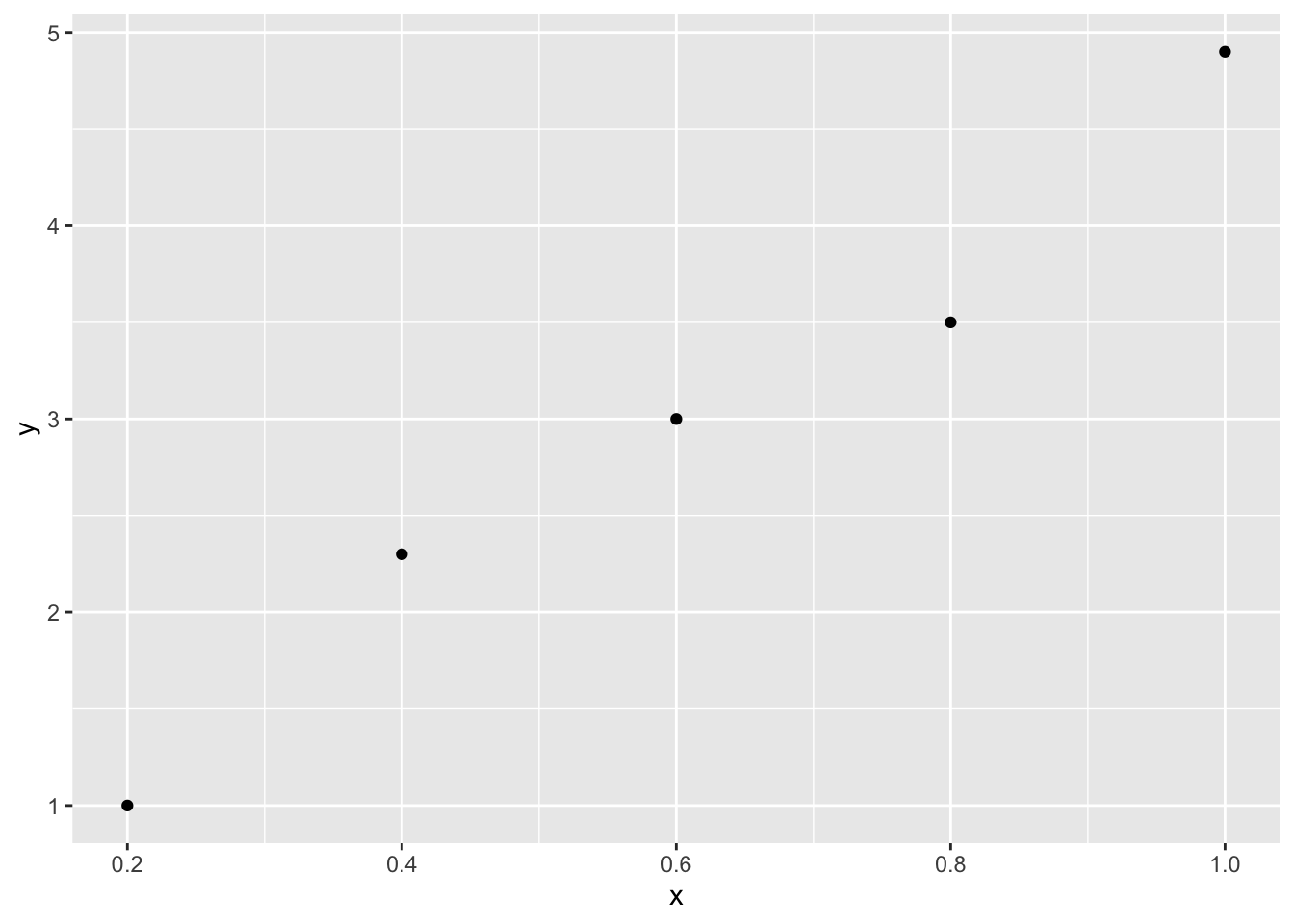
beta_1 <- cov(x, y) / var(x)
beta_1
## [1] 4.5beta_0 <- mean(y) - beta_1 * mean(x)
beta_0## [1] 0.24Properties
Let
\[X^n = (X_1, \dots, X_n)\] \[\beta = \begin{bmatrix} \beta_0 \\ \beta_1 \end{bmatrix}\]
Then,
\[E \left( \hat{\beta} |X^n\right) = \begin{bmatrix} \beta_0 \\ \beta_1 \end{bmatrix}\]
\[V \left( \hat{\beta} |X^n\right) = \frac{\sigma^2}{n s^2_x} \begin{bmatrix} \frac{1}{n}\sum_{i=1}^n X_i^2 & -\overline{X}_n \\ -\overline{X}_n & 1 \end{bmatrix}\]
where
\[s^2_x = \frac{\sum_{i=1}^n (X_i - \overline{X}_n)^2}{n}\]
The standard errors correspond to the diagonal terms of the matrix replacing \(\sigma\) by \(\hat\sigma\)
\[\hat{se}(\hat\beta_0 | X^n) = \frac{\hat\sigma}{s_x \sqrt{n}} \sqrt{\frac{\sum_{i=1}^nX_i^2}{n}}\] \[\hat{se}(\hat\beta_1 | X^n) = \frac{\hat\sigma}{s_x \sqrt{n}}\]
Consistency
\(\beta_0\) and \(\beta_1\) are consistent.
Asymptotic normality
\[\frac{\hat\beta_0 - \beta_0}{\hat{se}(\hat\beta_0)} \leadsto N(0,1)\] \[\frac{\hat\beta_1 - \beta_1}{\hat{se}(\hat\beta_1)} \leadsto N(0,1)\] #### \((1-\alpha)\) confidence intervals \[\hat\beta_0 \pm t_{\alpha/2} \hat{se}(\hat\beta_0)\] \[\hat\beta_1 \pm t_{\alpha/2} \hat{se}(\hat\beta_1)\]
Example
lm(y ~ x, data = dat) %>% confint()## 2.5 % 97.5 %
## (Intercept) -0.6881984 1.168198
## x 3.1006883 5.899312MLE
Theorem
If
\[\epsilon_i|X_i \sim N(0,\sigma^2)\]
The MLE estimates for the intercept and the slope are the least squares estimates and
\[\hat{\sigma} = \frac{SS_{res}}{n}\]
Demonstration
\[L(\theta|x,y)=f(x,y|\theta)\]
We don’t know the exact probability density functions for \(Y_1, Y_2,..,Y_n\) , but we know that for each \(Y_i\) the shape is the shape of the normal distribution centered around \(\mu_i = \beta_0+\beta_1x_i\). Then, the probability density function for \(Y_i\) is \[f(x_i,y_i\mid\theta)=f(x_i,y_i\mid \beta_0,\beta_1,\sigma)=\frac{1}{\sqrt{2\pi\sigma^2}}e^{-\frac{(y_i-\beta_0-\beta_1x_i)^2}{2\sigma^2}}\]
and the log likelihood \[log(L(\beta_0,\beta_1,\sigma))=-\frac{n}{2} log(2 \pi \sigma^2) - \frac{1}{2 \sigma^2} \sum_{i=1}^{n} (y_i-\beta_0-\beta_1 x_i)^2\]
It is clear that to maximize the likelihood we need to minimize the summation term, which actually corresponds to the least squares minimization. So the MLE intercept and slope corresponds to the typical regression model parameters. Introducing the best \(\beta_0\) \((\beta_{0MLE})\) and \(\beta_1\) \((\beta_{1MLE})\) and derivating relative to \(\sigma\) is easy to find the MLE for \(\sigma^{2}\) \[\sigma_{MLE}^{2}=\frac{1}{n} \sum_{i=1}^{n} (y_i-\beta_{0MLE}-\beta_{1MLE} x_i)^2=\frac{SS_{res}}{n}\]
Example
logL <- function(p) {
  n <- length(x) #A: p[1],  B: p[2],  sigma: p[3]
  -.5 * n * log(2 * pi * p[3]^2) -1 / (2 * p[3]^2) * sum((y - p[1]-p[2] * x)^2)
  }
negLogL <- function(x) -logL(x)
MLEparameters <- optim(c(0, 1, .1), negLogL)$par
MLEparameters## [1] 0.2407149 4.4988915 0.2153094xSeq <- seq(0,1,.1)
yPred <- MLEparameters[1] + MLEparameters[2] * xSeq
curveMLE <- data.frame(xSeq, yPred)
p + geom_line(data = curveMLE, aes(x = xSeq, y = yPred))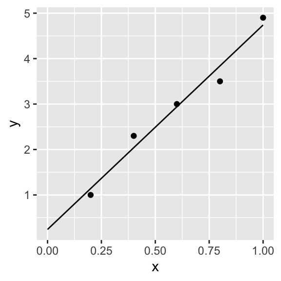
We can calculate which is the likelihood for the best parameters
logL(MLEparameters)## [1] 0.5814404Of course, we can estimate the parameters and the likelihood more directly
lm(y ~ x)##
## Call:
## lm(formula = y ~ x)
##
## Coefficients:
## (Intercept) x
## 0.24 4.50logLik(lm(y ~ x))## 'log Lik.' 0.5814469 (df=3)\(R^2\)
Definition
\[R^2 = 1 - \frac{SS_{res}}{SS_{tot}}\]
with
\[SS_{tot} = \sum_i (Y_i - \overline{Y})^2\]
It corresponds to the amount of variance explained and it could be calculated squaring the pearson coeeficient of correlation
\[R^2 = r^2\]
Exampple
ss_res <- (dat$y - beta_0 - beta_1 * dat$x)^2 %>% sum()
ss_tot <- (dat$y - mean(dat$y))^2 %>% sum()

1 - ss_res / ss_tot
## [1] 0.9721555Using lm
lm(y ~ x, data = dat) %>% summary() %>% .$r.square## [1] 0.9721555Adjusted \(R^2\)
\[R_{adj}^2 = 1 - \left( \frac{SS_{res}}{SS_{tot}} \times \frac{N-1}{N-K-1}\right) \]
where \(k\) is the number of predictors.
It take into account that adding more predictor will increas \(R^2\).
Example
1 - (ss_res / ss_tot * (length(dat$y) - 1) / (length(dat$y) -1 - 1) )## [1] 0.9628741Using lm
lm(y ~ x, data = dat) %>% summary() %>% .$adj.r.square## [1] 0.9628741Testing against the null model
\[H_0: \,Y_i = b_0+\epsilon_i\] \[H_1: \,Y_i = \sum_{k=1}^Kb_kX_{ik}+b_0+\epsilon_i\]
We need to use \(F\)
\[F = \frac{MS_{mod}}{MS_{res}}\]
with
\[MS_{mod}=\frac{SS_{mod}}{df_{mod}},\,\,MS_{res}=\frac{SS_{res}}{df_{res}},\,\,SS_{mod} =SS_{tot}-SS_{res} \]
and with \(df_{mod}=K\) and \(df_{res}=N-K-1\).
Example
ms_mod <- (ss_tot - ss_res) / 1

ms_res <- ss_res / (length(y) - 1 - 1)

ms_mod / ms_res
## [1] 104.7414Using lm
lm(y ~ x, data = dat) %>% summary() %>% .$fstatistic## value numdf dendf
## 104.7414 1.0000 3.0000Testing the individual coefficients
Given that the coefficients are asymptotically normal, a
t statistics is used
\[t = \frac{\hat{\beta_1}}{se(\hat{\beta_1})}\]
The formula of \(se(\hat{\beta_1})\) is not shown.
The test on the coefficients is the same that a test for correlation.
Example
lm(y ~ x, data = dat) %>% summary()##
## Call:
## lm(formula = y ~ x, data = dat)
##
## Residuals:
## 1 2 3 4 5
## -0.14 0.26 0.06 -0.34 0.16
##
## Coefficients:
## Estimate Std. Error t value Pr(>|t|)
## (Intercept) 0.2400 0.2917 0.823 0.47089
## x 4.5000 0.4397 10.234 0.00199 **
## ---
## Signif. codes: 0 '***' 0.001 '**' 0.01 '*' 0.05 '.' 0.1 ' ' 1
##
## Residual standard error: 0.2781 on 3 degrees of freedom
## Multiple R-squared: 0.9722, Adjusted R-squared: 0.9629
## F-statistic: 104.7 on 1 and 3 DF, p-value: 0.001989The slope is significant.