PCA

Theory

Data matrix

I have a data matrix \(X\) with \(n\) rows (number of observations) and \(p\) columns (number of features) with column-wise zero empirical mean. We don’ have response variable \(Y\).

Each row of \(X\) (observation), \(\vec{x}_{(i)} = (x_1, \dots, x_p)_{(i)}\), is a vector in a \(p\)-dimensional space.

Definition of PCA

PCA is defined as an orthogonal linear transformation of the data to a new coordinate system such that

the first coordinate (called the first principal component) is the coordinate for which the variance of the projection of the observations into the axis is the greatest
the second coordinate (called the second principal component) is the coordinate for which the variance of the projection of the observations into the axis is the second greatest
and so on.

The new coordinate system

The new coordinate system is defined by the vectors of weights or loadings

\[ \vec{w}_{(k)} = (w_1, \dots, w_p)_{(k)} \quad \text{for} \quad k=1 \dots m\]

Vector of principal components scores

The vector of principal components scores, \(\vec{t}_{(i)} = (t_1, \dots, t_m)_{(i)}\), is the map of the vector \(\vec{x}_{(i)}\) in the new coordinate system.

For a given observation \(\vec{x}_{(i)}\), the \(k\) score is given by the projection of \(\vec{x}_{(i)}\) over \(\vec{w}_{(k)}\)

\[t_{k(i)} = \vec{x}_{(i)} \cdot \vec{w}_{(k)} \quad \text{for} \quad i=1 \dots n \qquad k=1 \dots m \]

Matrix notation

If \(W\) is a matrix in which column \(k\) is \(\vec{w}_{(k)}\) and \(T\) is matrix in which each row is \(t_{(i)}\), then

\[T = X \cdot W\]

How to find the loadings?

It could be demonstrated that the loadings are the eigenvectors of \(X^T X\) ordered from decreasing value of the eigenvalue.

The loadings are unit vectors.

Simple example

We create a data matrix

library(tidyverse)

set.seed(40)
X <- tibble(x = seq(-6, 6, 2), y = x) %>%
  rowwise() %>% 
  mutate(x = x + rnorm(1), y = y + rnorm(1)) %>% 
  ungroup() %>% 
  mutate(x = x - mean(x), y = y - mean(y)) %>% 
  as.matrix()

dim(X)

## [1] 7 2

##               x             y
## 1 -6.000000e+00 -6.000000e+00
## 2 -4.000000e+00 -4.000000e+00
## 3 -2.000000e+00 -2.000000e+00
## 4  5.551115e-17 -1.110223e-16
## 5  2.000000e+00  2.000000e+00
## 6  4.000000e+00  4.000000e+00
## 7  6.000000e+00  6.000000e+00

p <- ggplot(X %>% as_tibble(), aes(x,y)) +
  geom_point() +
  coord_equal()
p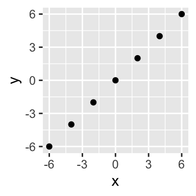

We use prcomp to calculate the loadings

pr <- prcomp(X, center = FALSE, scale = FALSE)

w <- pr$rotation


w_plot <- as_tibble(t(w)) %>% 
  bind_cols(tibble(component = rownames(t(w))))
                 

p + geom_segment(data = w_plot, 
                 aes(x = 0, y = 0, xend = x, yend = y, color = component),
                 arrow = arrow(length = unit(0.05, "npc"))) +
  scale_color_discrete(name = "loadings", 
                       breaks = c("PC1", "PC2"), 
                       labels = c(expression(bold(w)[(1)]), 
                                  expression(bold(w)[(2)]))) +
  coord_equal()

## Coordinate system already present. Adding new coordinate system, which will replace the existing one.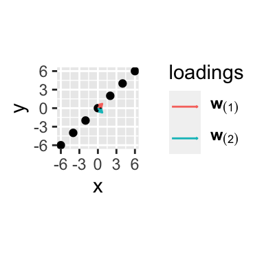

We calculate the principal components scores using the loadings

X %*% w

##             PC1          PC2
## 1 -8.485281e+00 0.000000e+00
## 2 -5.656854e+00 0.000000e+00
## 3 -2.828427e+00 0.000000e+00
## 4 -3.925231e-17 1.177569e-16
## 5  2.828427e+00 0.000000e+00
## 6  5.656854e+00 0.000000e+00
## 7  8.485281e+00 0.000000e+00

and check that corresponds to the principal components scores given directly by prcomp

pr$x

##             PC1          PC2
## 1 -8.485281e+00 0.000000e+00
## 2 -5.656854e+00 0.000000e+00
## 3 -2.828427e+00 0.000000e+00
## 4 -3.925231e-17 1.177569e-16
## 5  2.828427e+00 0.000000e+00
## 6  5.656854e+00 0.000000e+00
## 7  8.485281e+00 0.000000e+00

X %*% w == pr$x

##    PC1  PC2
## 1 TRUE TRUE
## 2 TRUE TRUE
## 3 TRUE TRUE
## 4 TRUE TRUE
## 5 TRUE TRUE
## 6 TRUE TRUE
## 7 TRUE TRUE

We plot the the scores in the new coordinate system

ggplot(pr$x %>% as_tibble(), aes(PC1, PC2)) +
  geom_point() +
  coord_equal()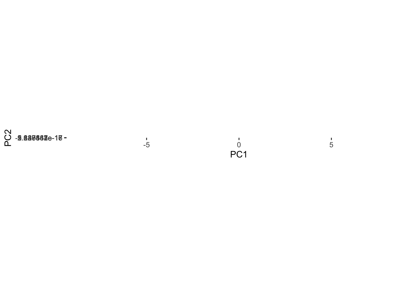

Checking centering and scaling in `prcomp`

library(tidyverse)

iris_center_scale <- iris %>% 
  mutate_if(is.numeric, funs( (. - mean(.)) / sd(.)))

## Warning: funs() is soft deprecated as of dplyr 0.8.0
## Please use a list of either functions or lambdas: 
## 
##   # Simple named list: 
##   list(mean = mean, median = median)
## 
##   # Auto named with `tibble::lst()`: 
##   tibble::lst(mean, median)
## 
##   # Using lambdas
##   list(~ mean(., trim = .2), ~ median(., na.rm = TRUE))
## This warning is displayed once per session.

# we check that is properly centered and scaled 
iris_center_scale %>% summarise_if(is.numeric, funs(mean, sd))

##   Sepal.Length_mean Sepal.Width_mean Petal.Length_mean Petal.Width_mean
## 1     -4.484318e-16     2.034094e-16     -2.895326e-17    -2.989362e-17
##   Sepal.Length_sd Sepal.Width_sd Petal.Length_sd Petal.Width_sd
## 1               1              1               1              1

PCA is the centered and scaled data

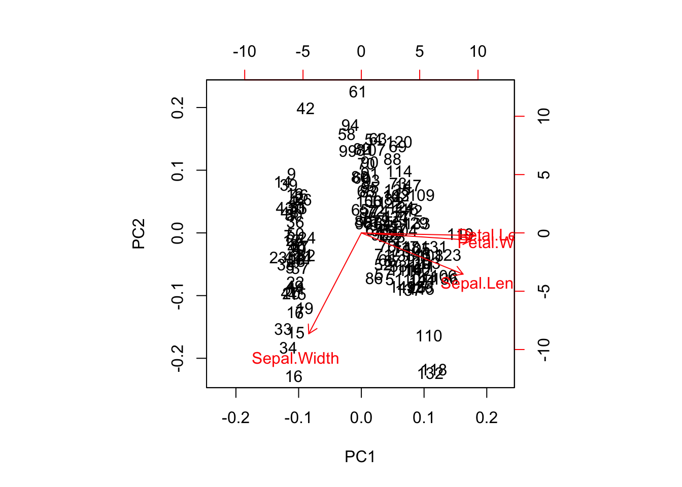
prcomp(iris_center_scale[-5], scale = FALSE, center = FALSE) %>% 
  biplot()

PCA automatically centering and scaling

prcomp(iris[-5], scale = TRUE, center = TRUE) %>% 
  biplot()

PCA