MLE for the binomial distribution and psychometric functions
library(tidyverse)The binomial distribution is defined as
\[f(x; \theta) = f(k; n, p) = \binom{n}{k} p^k (1-p)^{n-k}\]
where \(n\) is often fixed. Let’s consider that is 40. So we have \(f(k; p)\).
The problem in Probability theory
The parameter \(p\) is given and we can calculate the value of \(f\) for each posible value of \(k\).
Example 1:
Given \(p = 0.05\), the value of \(f\) for \(k=2\)?
\(f(k = 2; p = 0.05) = \binom{40}{2} 0.05^2 (1-0.05)^{38}\)
dbinom(x = 2, size = 40, prob = 0.05)## [1] 0.2776717Example 2:
Given \(p = 0.05\), the value of \(f\) for \(k=13\)?
dbinom(x = 13, size = 40, prob = 0.05)## [1] 3.677303e-08Example 3:
Given \(p = 0.25\), the value of \(f\) for \(k=13\)?
dbinom(x = 13, size = 40, prob = 0.25)## [1] 0.07590252The problem in Statistics
The problem in statistics is the inverse. The value of \(k\) is given and we want to estimate \(p\).
The typical experiment to introduce the binomial distribution is about flipping coins, but let’s use a detection experiment instead
- n: number of trials (40)
- k: number of times that the participant detects the stimulus
- p: probability of detection
Point estimation
The value of \(k\) is given and we want to estimate \(p\)
The typical solution is to choose \(p\) for which \(f\) is maximum (maximun likelihood estimation, MLE). The MLE of \(p\) is typically written as \(\hat{p}\).
When considering \(f\) as a function of \(p\), \(f\) is called likelihood \(L(p)\)
Let’s plot it for \(k=3\)
lik_fun <- function(p) dbinom(x = 3, size = 40, prob = p)

tibble(p = seq(0, 1, .001)) |>
  mutate(lik = lik_fun(p)) |>
  ggplot(aes(p, lik)) +
geom_line() 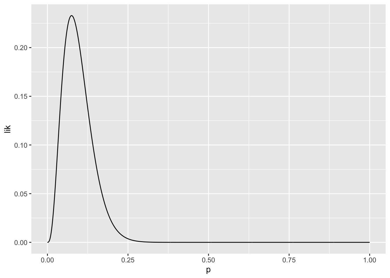
To find the maximum we calculate
\(\frac{dL}{dp} = 0\)
It could be demonstrated that the for binomial distribution \(\hat{p} = \frac{k}{n}\)
For example, for \(k=3\), \(\hat{p}\) ?
3/40## [1] 0.075Statistical model which is the product of two binomial distributions
\(f(k_1, k_2; p_1,p_2) = \binom{n}{k_1} {p_1}^{k_1} (1-p_1)^{n-k_1}\binom{n}{k_2} {p_2}^{k_2} (1-p_2)^{n-k_2}\)
Example:
In 40 trials where the probability was \(p_1\), \(k_1 =3\)
In 40 trials where the probability was \(p_2\), \(k_2 =16\)
\(L(3, 16;p_1, p_2)\)
The MLE of \(p_1\)
3/40## [1] 0.075The MLE of \(p_2\)
16/40## [1] 0.4Statistical model which is the product of five binomial distributions
\[f(k_1, \cdots,k_5; p_1,\cdots,p_5) = \prod_{i=1}^{5} \binom{n}{k_i} {p_i}^{k_i} (1-p_i)^{n-k_i}\]
Example
dat <- tibble(k = c(2, 16, 26, 32, 38), n = 40)
dat
## # A tibble: 5 × 2
## k n
## <dbl> <dbl>
## 1 2 40
## 2 16 40
## 3 26 40
## 4 32 40
## 5 38 40\(L(2, 16, 26, 32, 38; p_1, p_2, p_3, p_4,p_5)\)
dat <- dat |>
  mutate(p_mle = k /n)

dat
## # A tibble: 5 × 3
## k n p_mle
## <dbl> <dbl> <dbl>
## 1 2 40 0.05
## 2 16 40 0.4
## 3 26 40 0.65
## 4 32 40 0.8
## 5 38 40 0.95We have a model with
- 5 observations
- 5 parameters
A model in which we have a parameter for every observation is called the saturated model.
It is the maximum overfitting that we can do.
Because the likelihood involves many multiplications and it is very small, usually we use the logarithm of the likelihood. As the log likelihood is a monotonic transformation of the likelihood, the maximum of the log likelihood is the same as the maximum of the likelihood.
\[L(p_1,\cdots,p_5) = \sum_{i=1}^{5} \left( log \binom{n}{k_i} + {k_i}log({p_i})+({n-k_i}) log (1-p_i) \right)\]
The log likelihood of the saturated model is (the binomical coefficient is typically dropped as it does not depend on the parameters and does not affect the maximum likelihood estimation)
log_lik_saturated_fun <- function(p) {

  # p <- pmax(pmin(p, 0.9999), 0.0001) # Very important if optimization is performed to avoid log(0) and log(1) !!
  sum(lchoose(dat$n, dat$k) + dat$k * log(p) + (dat$n - dat$k) * log(1 - p))
}
and the maximum likelihood of the saturated model is
log_lik_saturated_fun(dat$p_mle)## [1] -8.507216The models with less parameters will have a log likelihood smaller than this.
Psychometric funcion
We reduce the number of parameters by expressing \(p_i\) in terms of an indexing variable \(x_i\) and less parameters
\[p_i = \gamma +(1- \gamma - \lambda) F(x_i;\mu, \sigma)\]
Where \(F\) is a function with a sigmoidal shape and \(\gamma\) and \(\lambda\) are parameters that are used to adjust the range of the function.
This expression for \(p_i\) is called the psychometric function (it has 4 parameters)
Let’s fix \(\gamma=0\) and \(\lambda = 0\) (2 parameters)
\[p_i = \Phi(x_i;\mu, \sigma)\]
An example of \(F\) is the logistic function
tibble(x = seq(-5, 5, .01)) |>
  mutate(phi = 1 / (1 + exp(-1 - 2 * x))) |>
  ggplot(aes(x, phi)) +
  geom_line()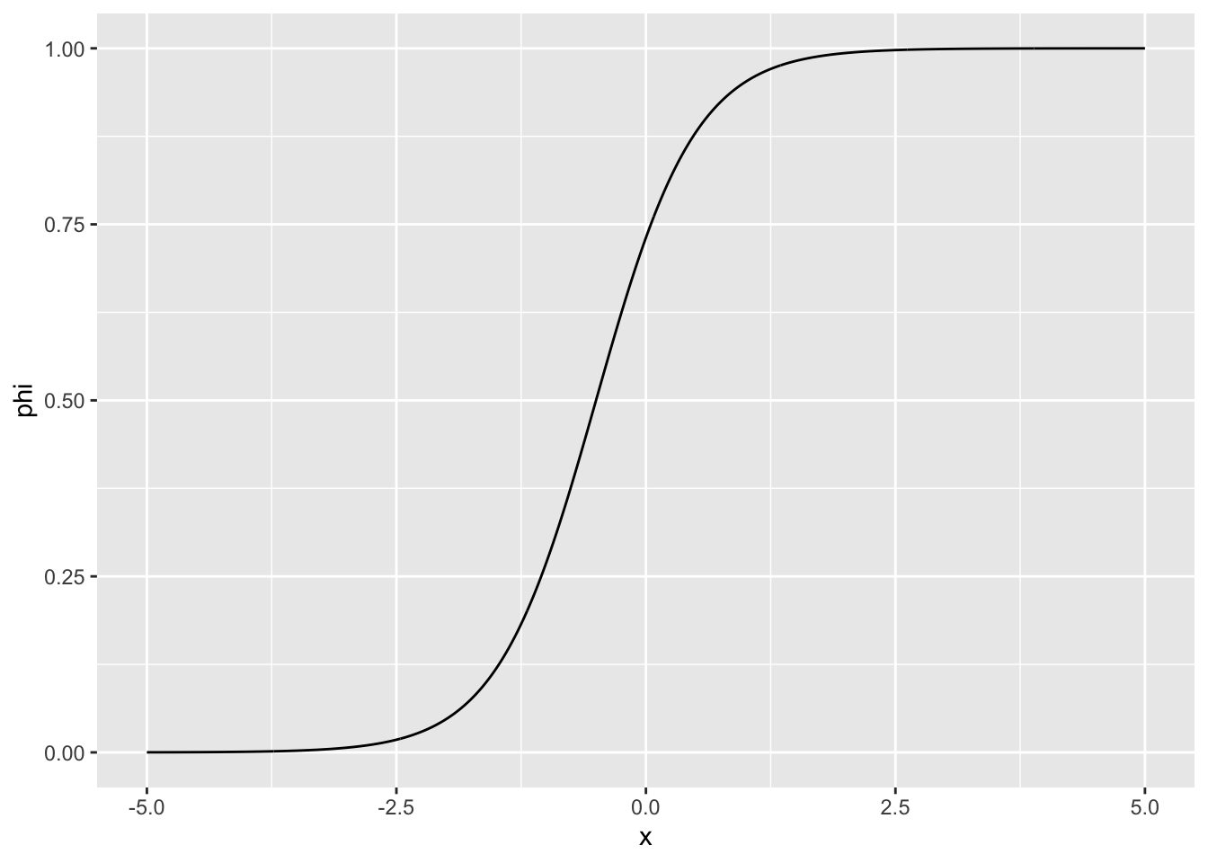
So the model we are fitting to the detection experiment is
\[f(k_1, \cdots,k_5; \mu, \sigma) = \prod_{i=1}^{5} \binom{n}{k_i} {\Phi(x_i;\mu, \sigma)}^{k_i} (1-\Phi(x_i;\mu, \sigma))^{n-k_i}\]
Let’s consider that our indexing variable is contrast
dat <- tibble(contrast = c(0, 1, 2, 3, 4), k = c(2, 16, 26, 32, 38), n = 40)

dat
## # A tibble: 5 × 3
## contrast k n
## <dbl> <dbl> <dbl>
## 1 0 2 40
## 2 1 16 40
## 3 2 26 40
## 4 3 32 40
## 5 4 38 40So we are hypothesizing that \(p_i\) increases with contrast.
We can plot \(k\) as a function of contrast
dat |>
  ggplot(aes(contrast, k)) +
  geom_point() +
  ylim(0,40)
or the probability of detecting (which indeed correspond to the best estimation of the parameters of the saturated model) as a function of contrast
dat <- dat|>
  mutate(p = k /n )

dat |>
  ggplot(aes(contrast, p)) +
  geom_point() +
  ylim(0,1)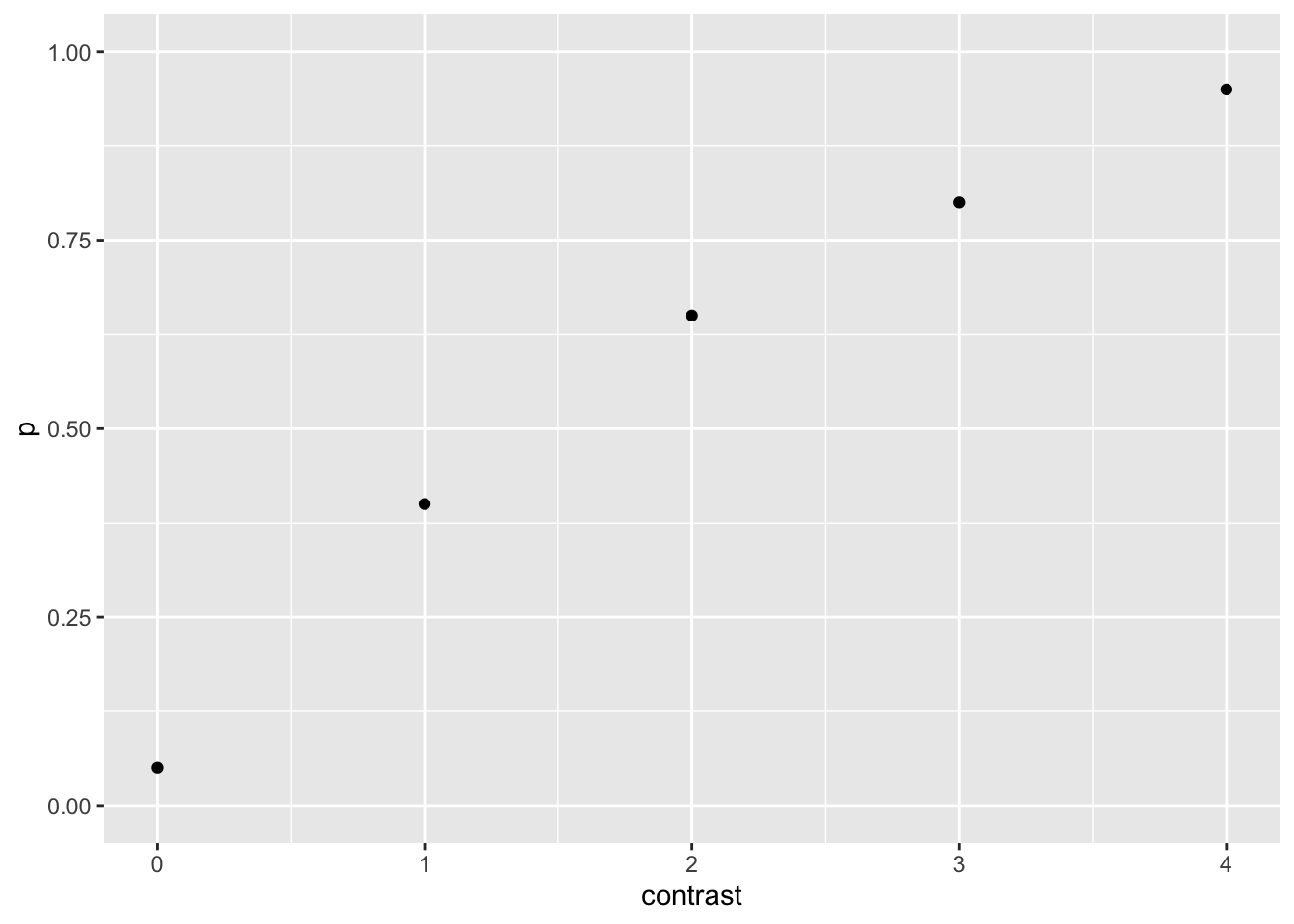
The log likelihood of tha saturated model was
log_lik_saturated_fun <- function(p) { # p is a vector of 5 parameters
  sum(lchoose(dat$n, dat$k) + dat$k * log(p) + (dat$n - dat$k) * log(1 - p))
}
and the log likelihood of the psychometric function model is
log_lik_fun <- function(p) { #p is a vector of 2 parameters: mu and sigma
  phi <-  1 / (1 + exp(-p[1] - p[2] * dat$contrast))
  sum(lchoose(dat$n, dat$k) + dat$k * log(phi) + (dat$n - dat$k) * log(1 - phi))
}
Let´s look at some log lik
log_lik_fun(c(3, 1))## [1] -264.8652log_lik_fun(c(1.5, 1))## [1] -145.7988Let’s find the values of \(p_1\) and \(p_2\) that maximize the log lik
neg_log_lik_fun <- function(p) -log_lik_fun(p)

mle_par <- optim(c(1, 1), neg_log_lik_fun)$par

mle_par
## [1] -2.018336 1.246996So the psychometric function is
psy_curve <- tibble(contrast = seq(0, 4, .1)) |>
  mutate(p =  1 / (1 + exp(-mle_par[1] - mle_par[2] * contrast)))
Let’s added to the previous plot
  ggplot() +
  geom_point(data = dat, aes(contrast, p)) +
  geom_line(data = psy_curve, aes(x = contrast, y = p)) +
  ylim(0,1)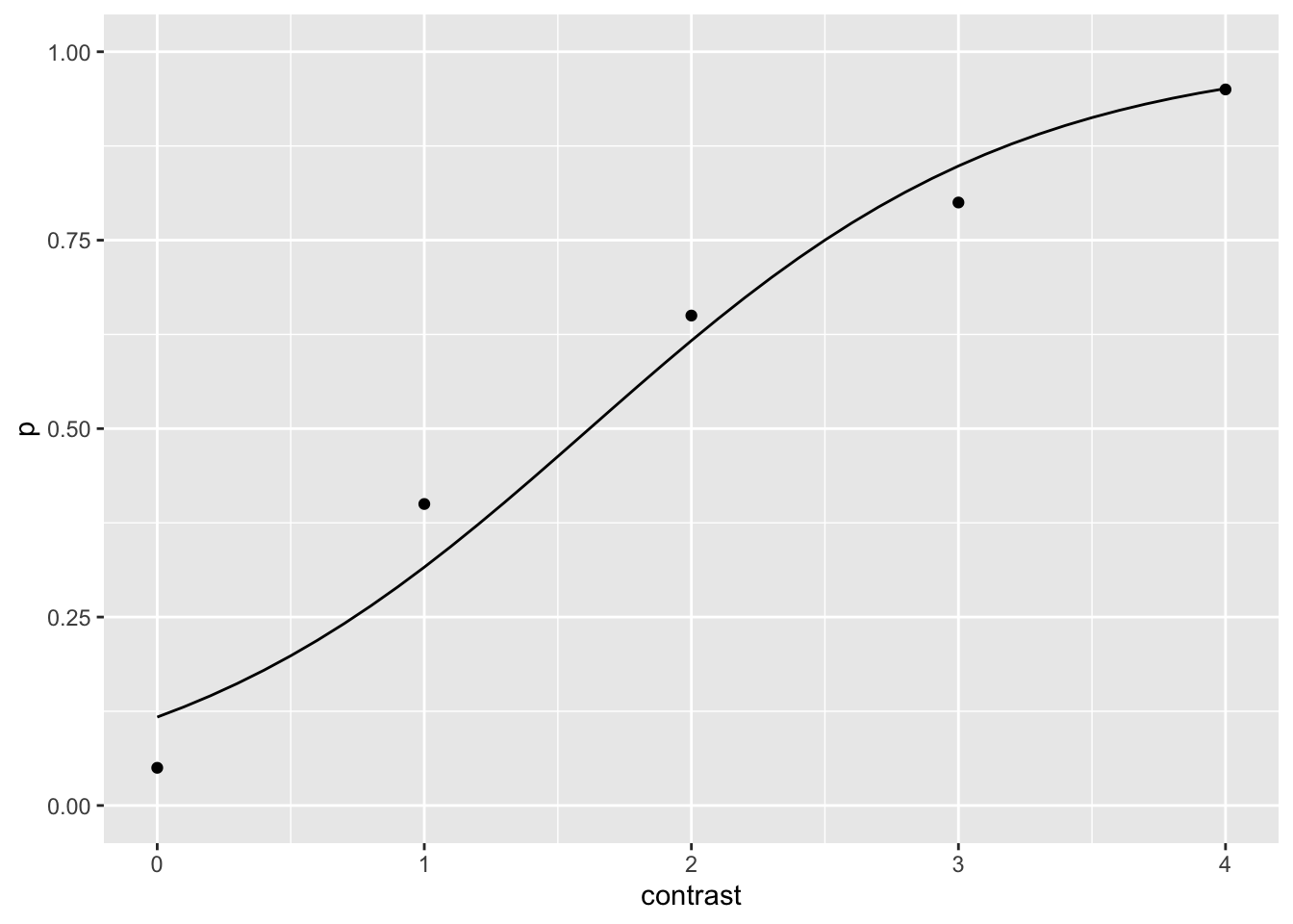
The likelihood of the model for the MLE parameters
log_lik_fun(mle_par)## [1] -10.65097