MLE for the normal distribution
This is an example to illustrate MLE. Actually, it could be easy demonstrated that when the parametric family is the normal density function, then the MLE of \(\mu\) is the mean of the observations and the MLE of \(\sigma\) is the uncorrected standard deviation of the observations.
Suppose that we have the following independent observations and we know that they come from the same probability density function
library(tidyverse)

x<- c(29, 41, 32, 28, 38) #our observations

dat <- tibble(x, y=0) #we plotted our observations in the x-axis
p <- ggplot(data = dat, aes(x = x, y = y)) + geom_point()
p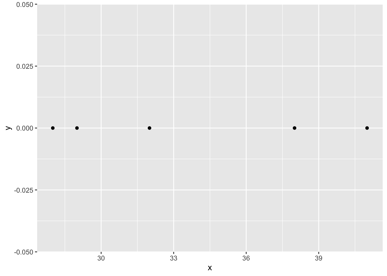
We don’t know the exact probability density function, but we know that the shape (the parametric family) is the shape of the normal density function \[f(x;\theta)=f(x;\mu,\sigma)=\frac{1}{\sqrt{2\pi\sigma^2}}e^{-\frac{(x-\mu)^2}{2\sigma^2}}\] Let’s plot two arbitrary probability density functions fixing the parameters of the parametric family
xseq <- seq(20, 45, .1)
f1 <- dnorm(xseq, 33, 7) #mu=33, sigma=7
f2 <- dnorm(xseq, 27, 4) #mu=27, sigma=4
curve1 <-tibble(xseq,f1)
curve2 <-tibble(xseq,f2)
p <- p +
geom_line(data = curve1, aes(x = xseq, y = f1)) +
geom_line(data = curve2, aes(x = xseq, y = f2))
p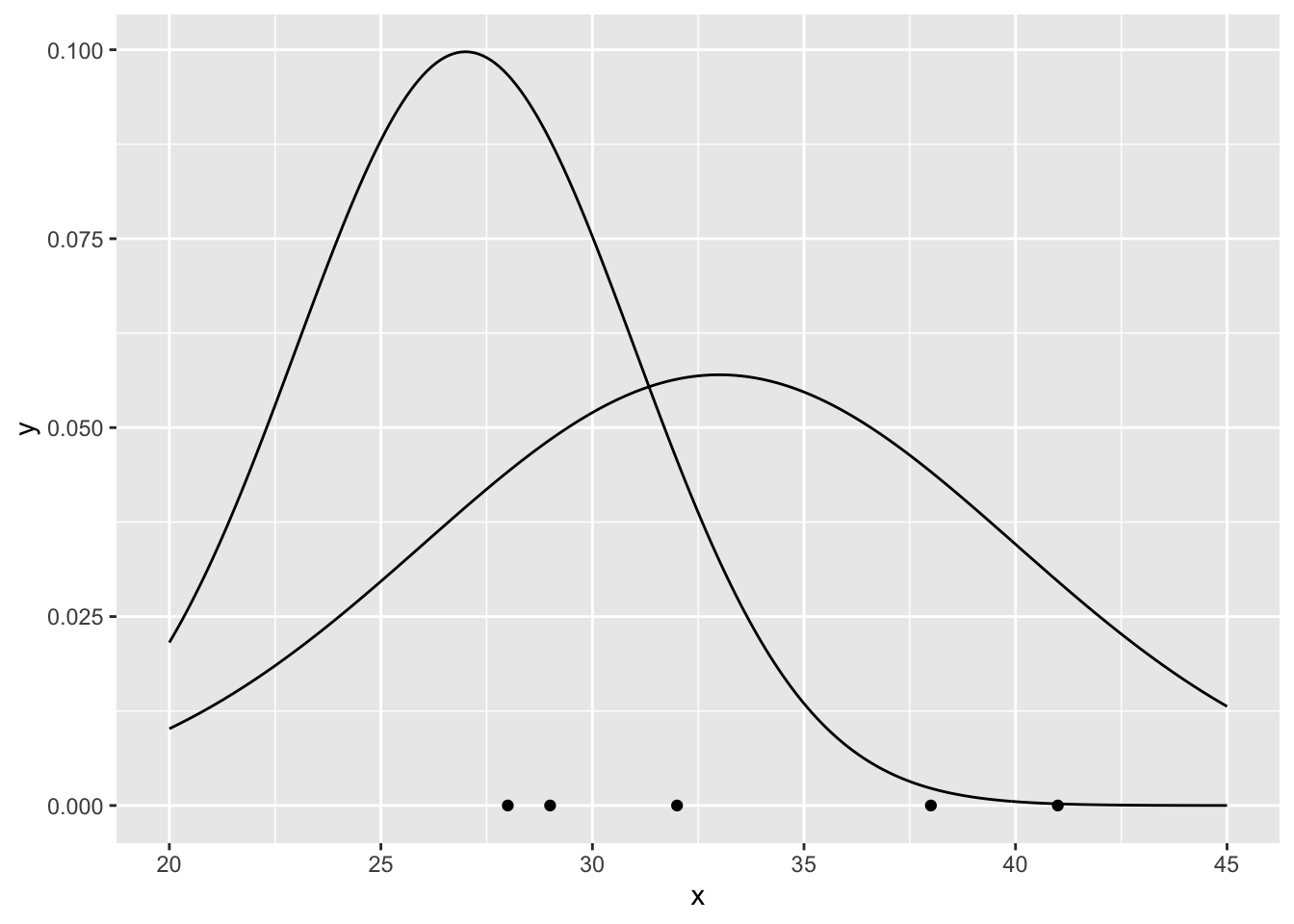 It is clear that the probability density function \(f\) for \(\mu=33\) and \(\sigma=7\) describes the observations better than the other one. We are interested in the \(f\) that maximizes \(L\).
The joint density function is \[f(x;\mu,\sigma)=f(x_1;\mu,\sigma)f(x_2;\mu,\sigma)...f(x_5;\mu,\sigma)=\] \[ =\frac{1}{\sqrt{2\pi\sigma^2}}e^{-\frac{(x_1-\mu)^2}{2\sigma^2}}\frac{1}{\sqrt{2\pi\sigma^2}}e^{-\frac{(x_2-\mu)^2}{2\sigma^2}}...\frac{1}{\sqrt{2\pi\sigma^2}}e^{-\frac{(x_5-\mu)^2}{2\sigma^2}}.\] that when considered as a function of the parameters is \[L(\mu,\sigma|x)=L(\mu,\sigma|29,41,32,28,38)=f(x|\mu,\sigma)=f(29,41,32,28,38|\mu,\sigma)=\] \[=f(29|\mu,\sigma)f(41|\mu,\sigma)...f(38|\mu,\sigma)=\] \[ =\frac{1}{\sqrt{2\pi\sigma^2}}e^{-\frac{(29-\mu)^2}{2\sigma^2}}\frac{1}{\sqrt{2\pi\sigma^2}}e^{-\frac{(41-\mu)^2}{2\sigma^2}}...\frac{1}{\sqrt{2\pi\sigma^2}}e^{-\frac{(38-\mu)^2}{2\sigma^2}}\]
and \[log(L)=log(f(x;\mu,\sigma))=log(f(x_1;\mu,\sigma))+log(f(x_2;\mu,\sigma))+...+log(f(x_5;\mu,\sigma))=\] \[=log(f(29;\mu,\sigma))+log(f(41;\mu,\sigma))+...+log(f(38;\mu,\sigma))\]
logL <- function(p) sum(log(dnorm(x, p[1], p[2]))) # p = c(p[1], p[2]) = c(mu, sigma)
#logL <-function(p) sum(dnorm(x, p[1], p[2],log = TRUE)) #alternative way to write it
We can calculate the \(log(L)\) for the two previous examples to verify that \(log(L)\) is larger for \(\mu=33\) and \(\sigma=7\)
logL(c(33, 7))## [1] -15.66098logL(c(27, 4))## [1] -22.36991logL(c(33, 7)) > logL(c(27,4))## [1] TRUELet’s plot the \(log(L)\) for some values of \(\mu\) and \(\sigma\)
dLogL <- crossing(museq = seq(20, 45, .1), sigmaseq = seq(4, 10, 1)) %>%
  rowwise() %>%
  mutate(logLike = logL(c(museq, sigmaseq)))


ggplot(data = dLogL,
       aes(x= museq, y=logLike, color = factor(sigmaseq))) +
  geom_line()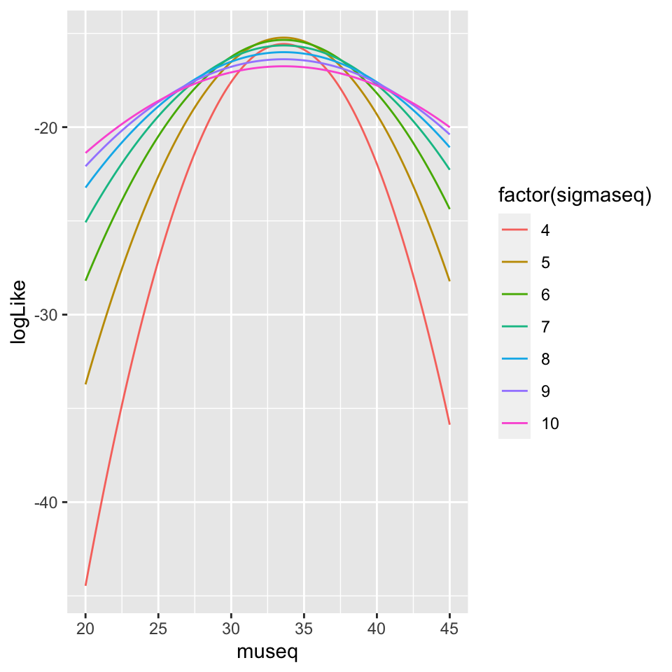
So it seems that values of \(\mu\) around 34 and \(\sigma\) around 5 maximizes log(L). Let’s maximize it properly using optim. Because optim search for a minimum, we need to minimize \(-log(L)\)
negLogL <- function(p) -logL(p)
estPar <- optim(c(20, 10), negLogL) # some initial parameters
MLEparameters <- estPar$par

MLEparameters
## [1] 33.598814 5.083355So, we found that from the parametric family, the probability density function that better characterizes the observations according to MLE is the one described by the parameters \(\mu=\) 33.5988136 and \(\sigma=\) 5.0833546. Let’s plot the distribution in red in the previous graph
fMLE <- dnorm(seq(20,45,.1), MLEparameters[1], MLEparameters[2])
curveMLE<-tibble(xseq, fMLE)

p + geom_line(data = curveMLE, aes(x = xseq, y = fMLE), color = "red")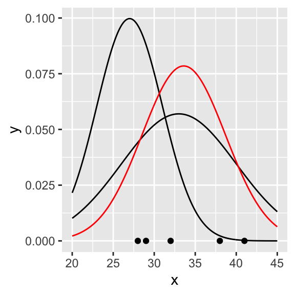
It could be easy demonstrated that actually when the parametric family is the normal density function, then the MLE of \(\mu\) is the mean of the observations
mean(x)## [1] 33.6and the MLE of \(\sigma\) is the uncorrected standard deviation of the observations
sqrt(mean((x - mean(x))^2))## [1] 5.083306