ANCOVA
library(tidyverse)
library(faraway)
dat <- teengamb %>%
mutate(sex = if_else(sex == 0, "male", "female"))
dat %>%
ggplot(aes(x = income, y = gamble, color = sex)) +
geom_point() 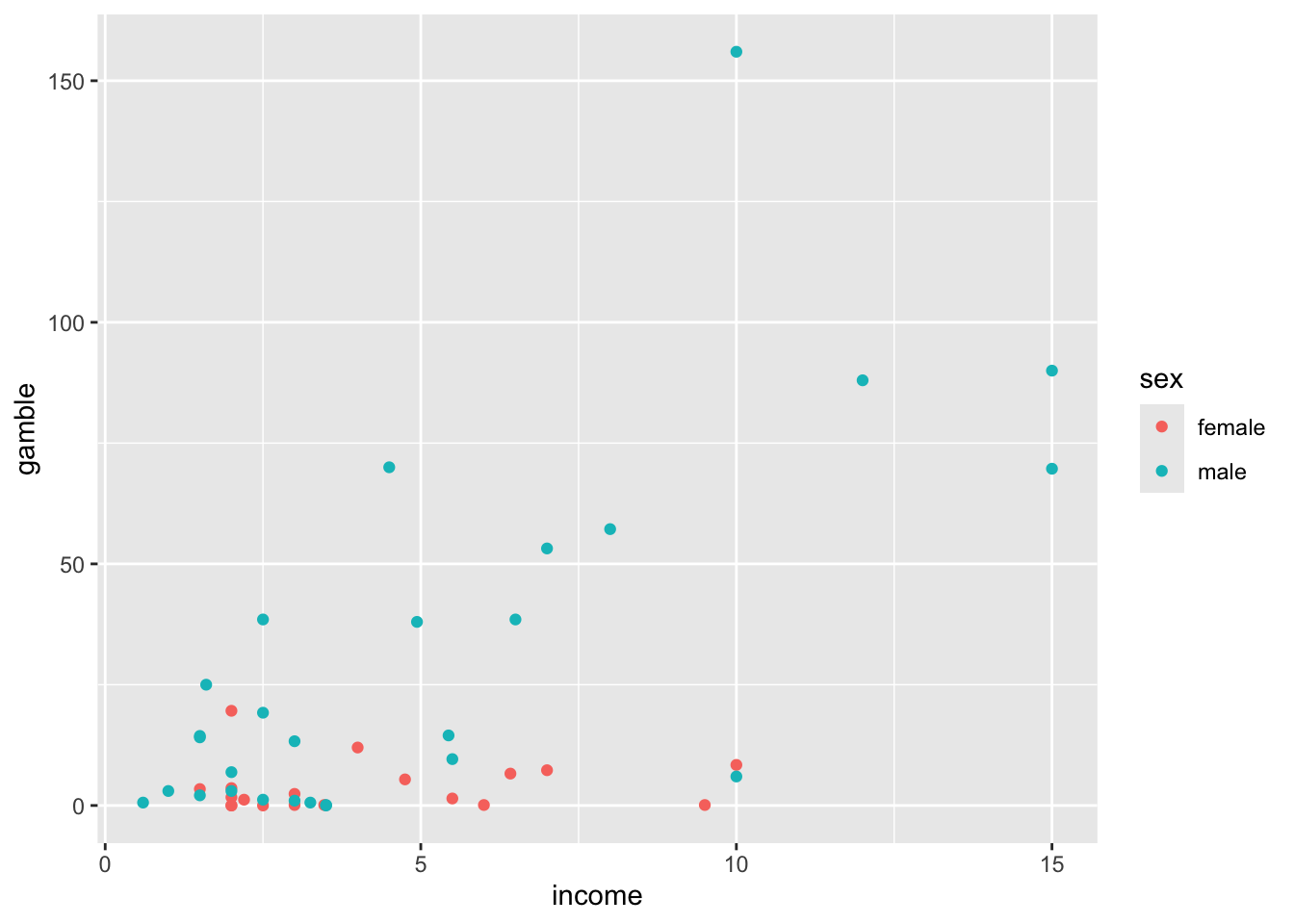
Least-square estimation for the model without interaction
create_least_squares <- function(d){

  indicator <- d %>%
    mutate(i = if_else(sex == "female", 0, 1)) %>%
    pull(i)

  function(p) {
  ypred <- p[1] + p[2] * indicator + d$income * p[3]
  sum((d$gamble - ypred)^2)
  }
}


least_squares_fun <- create_least_squares(dat)

ls_par <- optim(c(1, 1, 1), least_squares_fun)$par

dat %>%
  ggplot(aes(x = income, y = gamble, color = sex)) +
  geom_point() +
  geom_line(
    data = tibble(income = seq(0, 15, .1)) %>%
      mutate(gamble = ls_par[1] + income * ls_par[3]) %>%
      mutate(sex = "female")
  ) +
    geom_line(
    data = tibble(income = seq(0, 15, .1)) %>%
      mutate(gamble = ls_par[1] + ls_par[2] +income * ls_par[3]) %>%
      mutate(sex = "male")
  )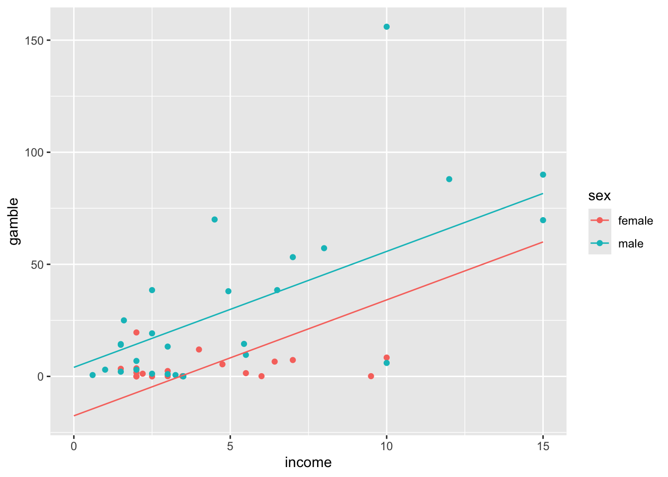
The parameters
ls_par## [1] -17.589709 21.629103 5.171457Using lm
lm_no_interaction <- lm(gamble ~ sex + income , data = dat)

summary(lm_no_interaction)
##
## Call:
## lm(formula = gamble ~ sex + income, data = dat)
##
## Residuals:
## Min 1Q Median 3Q Max
## -49.757 -11.649 0.844 8.659 100.243
##
## Coefficients:
## Estimate Std. Error t value Pr(>|t|)
## (Intercept) -17.594 6.544 -2.688 0.01010 *
## sexmale 21.634 6.809 3.177 0.00272 **
## income 5.172 0.951 5.438 2.24e-06 ***
## ---
## Signif. codes: 0 '***' 0.001 '**' 0.01 '*' 0.05 '.' 0.1 ' ' 1
##
## Residual standard error: 22.75 on 44 degrees of freedom
## Multiple R-squared: 0.5014, Adjusted R-squared: 0.4787
## F-statistic: 22.12 on 2 and 44 DF, p-value: 2.243e-07Design-matrix
model.matrix(lm_no_interaction)## (Intercept) sexmale income
## 1 1 0 2.00
## 2 1 0 2.50
## 3 1 0 2.00
## 4 1 0 7.00
## 5 1 0 2.00
## 6 1 0 3.47
## 7 1 0 5.50
## 8 1 0 6.42
## 9 1 0 2.00
## 10 1 0 6.00
## 11 1 0 3.00
## 12 1 0 4.75
## 13 1 0 2.20
## 14 1 0 2.00
## 15 1 0 3.00
## 16 1 0 1.50
## 17 1 0 9.50
## 18 1 0 10.00
## 19 1 0 4.00
## 20 1 1 3.50
## 21 1 1 3.00
## 22 1 1 2.50
## 23 1 1 3.50
## 24 1 1 10.00
## 25 1 1 6.50
## 26 1 1 1.50
## 27 1 1 5.44
## 28 1 1 1.00
## 29 1 1 0.60
## 30 1 1 5.50
## 31 1 1 12.00
## 32 1 1 7.00
## 33 1 1 15.00
## 34 1 1 2.00
## 35 1 1 1.50
## 36 1 1 4.50
## 37 1 1 2.50
## 38 1 1 8.00
## 39 1 1 10.00
## 40 1 1 1.60
## 41 1 1 2.00
## 42 1 1 15.00
## 43 1 1 3.00
## 44 1 1 3.25
## 45 1 1 4.94
## 46 1 1 1.50
## 47 1 1 2.50
## attr(,"assign")
## [1] 0 1 2
## attr(,"contrasts")
## attr(,"contrasts")$sex
## [1] "contr.treatment"Least-square estimation for the model with interaction
create_least_squares_with_interaction <- function(d){
indicator <- d %>%
mutate(i = if_else(sex == "female", 0, 1)) %>%
pull(i)
function(p) {
ypred <- p[1] + p[2] * indicator + d$income * (p[3] + indicator * p[4])
sum((d$gamble - ypred)^2)
}
}
least_squares_with_interaction_fun <- create_least_squares_with_interaction(dat)
ls_par_int <- optim(c(1, 1, 1, 1), least_squares_with_interaction_fun)$par
dat %>%
ggplot(aes(x = income, y = gamble, color = sex)) +
geom_point() +
geom_line(
data = tibble(income = seq(0, 15, .1)) %>%
mutate(gamble = ls_par_int[1] + income * ls_par_int[3]) %>%
mutate(sex = "female")
) +
geom_line(
data = tibble(income = seq(0, 15, .1)) %>%
mutate(gamble = ls_par_int[1] + ls_par_int[2] +
income * (ls_par_int[3] + ls_par_int[4])) %>%
mutate(sex = "male")
)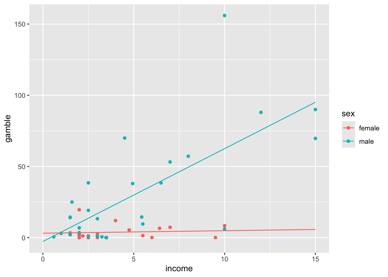 The parameters
ls_par_int## [1] 3.1471640 -5.8155537 0.1748834 6.3432484Using lm
lm_interaction <- lm(gamble ~ sex * income, data = dat)

summary(lm_interaction)
##
## Call:
## lm(formula = gamble ~ sex * income, data = dat)
##
## Residuals:
## Min 1Q Median 3Q Max
## -56.522 -4.860 -1.790 6.273 93.478
##
## Coefficients:
## Estimate Std. Error t value Pr(>|t|)
## (Intercept) 3.1400 9.2492 0.339 0.73590
## sexmale -5.7996 11.2003 -0.518 0.60724
## income 0.1749 1.9034 0.092 0.92721
## sexmale:income 6.3432 2.1446 2.958 0.00502 **
## ---
## Signif. codes: 0 '***' 0.001 '**' 0.01 '*' 0.05 '.' 0.1 ' ' 1
##
## Residual standard error: 20.98 on 43 degrees of freedom
## Multiple R-squared: 0.5857, Adjusted R-squared: 0.5568
## F-statistic: 20.26 on 3 and 43 DF, p-value: 2.451e-08Design-matrix
model.matrix(lm_interaction)## (Intercept) sexmale income sexmale:income
## 1 1 0 2.00 0.00
## 2 1 0 2.50 0.00
## 3 1 0 2.00 0.00
## 4 1 0 7.00 0.00
## 5 1 0 2.00 0.00
## 6 1 0 3.47 0.00
## 7 1 0 5.50 0.00
## 8 1 0 6.42 0.00
## 9 1 0 2.00 0.00
## 10 1 0 6.00 0.00
## 11 1 0 3.00 0.00
## 12 1 0 4.75 0.00
## 13 1 0 2.20 0.00
## 14 1 0 2.00 0.00
## 15 1 0 3.00 0.00
## 16 1 0 1.50 0.00
## 17 1 0 9.50 0.00
## 18 1 0 10.00 0.00
## 19 1 0 4.00 0.00
## 20 1 1 3.50 3.50
## 21 1 1 3.00 3.00
## 22 1 1 2.50 2.50
## 23 1 1 3.50 3.50
## 24 1 1 10.00 10.00
## 25 1 1 6.50 6.50
## 26 1 1 1.50 1.50
## 27 1 1 5.44 5.44
## 28 1 1 1.00 1.00
## 29 1 1 0.60 0.60
## 30 1 1 5.50 5.50
## 31 1 1 12.00 12.00
## 32 1 1 7.00 7.00
## 33 1 1 15.00 15.00
## 34 1 1 2.00 2.00
## 35 1 1 1.50 1.50
## 36 1 1 4.50 4.50
## 37 1 1 2.50 2.50
## 38 1 1 8.00 8.00
## 39 1 1 10.00 10.00
## 40 1 1 1.60 1.60
## 41 1 1 2.00 2.00
## 42 1 1 15.00 15.00
## 43 1 1 3.00 3.00
## 44 1 1 3.25 3.25
## 45 1 1 4.94 4.94
## 46 1 1 1.50 1.50
## 47 1 1 2.50 2.50
## attr(,"assign")
## [1] 0 1 2 3
## attr(,"contrasts")
## attr(,"contrasts")$sex
## [1] "contr.treatment"